Getting started in ten minutes

One equation, one plot, one physical number. You write the viscous Burgers equation as on paper, simulate it, draw the solution and measure its kinetic energy, which the script checks against the exact solution. Then four small changes show what Conatus decides for you, and what it never does. The longer path through one problem, from stability to a simulation of convection rolls, is 0. Getting started: convection between two plates.

Time: ten minutes; the script runs in a few seconds. Script: t00_first_steps.py.

Install

python3.12 -m venv venv && . venv/bin/activate
pip install "conatus[tutorials]"
python -m conatus doctor

The last line says what this machine can run; Installation has the other ways to install.

The equation

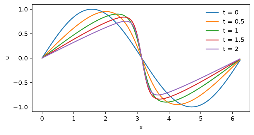
A wave \(u(x, t)\) on a periodic line of length \(2\pi\) steepens under its own advection and is held back by viscosity \(\nu\):

\[ \partial_t u + u\,\partial_x u = \nu\,\partial_x^2 u, \qquad u(x, 0) = \sin x . \]

import numpy as np

import conatus as cn

m = cn.Model(cn.Box(x=cn.periodic(2 * np.pi)), name="Burgers", nu=0.1)
m.scalar("u")
m.equations("dt(u) - nu*lap(u) = -u*dx(u)")
print(m.explain())

The domain, the unknown, the parameter and the equation are all you write. m.explain() prints what Conatus decided from them: the linear term is treated implicitly, the product u*dx(u) explicitly, and the product is dealiased by the 3/2 rule.

Time stepping: 2 linear term(s) implicit; nonlinear terms explicit (eq0)
Dealiasing: x: 3/2 (declared default for products of degree 2)

Simulate and plot

sim = m.simulate(N=128, scheme="RK443", dt=1e-3)    # resolution, scheme, time step: your choices
sim.initial(u=lambda x: np.sin(x))
x = sim.coordinate("x")
profiles = {}
for t in (0.0, 0.5, 1.0, 1.5, 2.0):
    if t > sim.t:
        sim.run(until=t)
    profiles[t] = sim.grid("u").copy()

A simulation needs a resolution, a scheme and a time step: three arguments, never defaults. run(until=t) advances to \(t\), which must be a whole number of steps: the step is never changed for you.

import os

import matplotlib.pyplot as plt

fig, ax = plt.subplots(figsize=(6.4, 3.2), dpi=150)
for t, ut in profiles.items():
    ax.plot(x, ut, label=f"t = {t:g}")
ax.set_xlabel("x")
ax.set_ylabel("u")
ax.legend(frameon=False)
out = os.environ.get("CN_TUTORIAL_OUT", ".")
os.makedirs(out, exist_ok=True)
fig.savefig(os.path.join(out, "burgers.png"), bbox_inches="tight")

One physical number

The kinetic energy \(E = \tfrac12 \int u^2\,dx\) starts at \(\pi/2\) and decreases as viscosity dissipates the steepening front.

u = sim.grid("u")
energy = np.pi * np.mean(u**2)                     # E = 1/2 int u^2 dx (grid mean, exact here)
print(f"kinetic energy at t = {sim.t:g}: E = {energy:.12f} (E(0) = pi/2 = {np.pi / 2:.12f})")

The Cole–Hopf transformation turns the Burgers equation into the heat equation, so the exact solution is known (Cole 1951; Hopf 1950). The script ends by comparing the energy with it:

kinetic energy at t = 2: E = 0.759907890109 (E(0) = pi/2 = 1.570796326795)
Cole-Hopf: E = 0.759907890081, relative error 3.7e-11
OK: the kinetic energy of the simulation equals the exact Cole-Hopf value

Four changes to try

Change one line of the script, run it again and read what happens.

1. Less viscosity. cn.Model(..., nu=0.05) makes the front twice as steep. The energy still matches the exact solution (change the 0.1 of cole_hopf_energy too), to \(2\times10^{-10}\).

2. Too few modes. m.simulate(N=32, ...) cannot resolve the front. Conatus does not raise the resolution for you: it warns, once, with an UnderResolvedWarning that names the unknown, the direction and the spectral tail, and the energy is then only right to about \(4\times10^{-6}\).

3. A larger time step. dt=0.05 takes 40 steps instead of 2000. The scheme is third order in time, so the energy error grows to about \(4\times10^{-6}\); sim.cfl(safety=0.5) tells you a stable step, it never imposes one.

4. Another equation. Drop the nonlinear term: m.equations("dt(u) - nu*lap(u) = 0") is the heat equation, and the energy decays exactly as \(E(t) = \tfrac{\pi}{2} e^{-2\nu t}\).

Next

0. Getting started: convection between two plates takes one problem, convection between two plates, from its equations to its stability, its onset and a simulation; then each tutorial of Tutorials ends on a published value.

Output

# t00_first_steps: PASS (exit 0) in 30.5 s | 2026-10-20 | script sha256 46b3ef78528aff94
Model 'Burgers': Box(x=periodic((0, 6.28319))) (Cartesian box)
Unknowns: u (scalar); parameters: nu = 0.1
Equations as written:
  eq0: dt(u) - nu*lap(u) = -u*dx(u)
Problem: IVP (a time derivative dt() appears)
Time stepping: 2 linear term(s) implicit; nonlinear terms explicit (eq0)
Dealiasing: x: 3/2 (declared default for products of degree 2)
Resolution: not chosen yet (simulate/eigenvalues/discretize(N=...))
(every decision, tau by tau and term by term: m.explain(full=True))
kinetic energy at t = 2: E = 0.759907890109 (E(0) = pi/2 = 1.570796326795)
Cole-Hopf: E = 0.759907890081, relative error 3.7e-11
OK: the kinetic energy of the simulation equals the exact Cole-Hopf value