13. Where a global mode is born, and what the data say about it

The adjoint tells where to act; the data, read in the right norm, tell what the operator predicts.

Goal. Compute the direct and adjoint global modes of the linear Ginzburg–Landau equation, its wavemaker (Giannetti & Luchini 2007) and the gradient of the eigenvalue with respect to the “base flow” μ(x) (Marquet, Sipp & Jacquin 2008); then decompose data produced by the same model: DMD of a transient. Expected. Wavemaker maximum S₀(0) = |χ|/√π and dλ₀/dμ₂ = 1/(4χ²) (closed forms, Chomaz 2005) to 1e-9; DMD returns the four least stable eigenvalues to 1e-9. Time: about 20 s of CPU. Script: t13_sensitivity_data.py · Tests behind it: tests/sensitivity/, tests/datadriven/. The Ginzburg–Landau model comes ready (linear_ginzburg_landau, expert layer): the sensitivity tools need it as a function of the “base flow” μ(x), which they differentiate.

The model

import numpy as np
import scipy.linalg as sla

from conatus.expert import (DataInnerProduct, Y, base_flow_sensitivity, dmd, ginzburg_landau_exact,
                            linear_ginzburg_landau, state_space,
                            structural_sensitivity)
from conatus.diagnostics import Chebyshev, Grid
# [/imports]

# [model]
NU, GAMMA, MU_C, MU_2 = 2 + 0.4j, 1 - 1j, 0.34, -0.01        # Bagheri et al. (2009)
BOUNDS = (-60.0, 60.0)                                     # the whole line, truncated (declared)


def gl(mu):
    """dq/dt = -nu q' + gamma q'' + mu(x) q, q = 0 at both ends; mu is a sympy expression in Y."""
    return linear_ginzburg_landau(nu=NU, gamma=GAMMA, mu=mu, bounds=BOUNDS)


MU = MU_C + MU_2 * Y ** 2 / 2
exact = ginzburg_landau_exact(nu=NU, gamma=GAMMA, mu_c=MU_C, mu2=MU_2, n=0)
print(exact.explain())

Structural and base-flow sensitivity

The adjoint is declared (adjoint="continuous": the formal adjoint with its checked boundary conditions); the product is the energy of the system; nothing is normalized for you without being said in explain().

bfs = base_flow_sensitivity(gl, MU, N=140, target=exact.eigenvalue, adjoint="continuous",
                            infinite_tol=1e-10, adjoint_bcs=[("q", 0, "left"), ("q", 0, "right")])
pair = bfs.pair
print(pair.explain())
st = structural_sensitivity(pair)
x_star, s_star = st.maximum(points=1201)
print(f"wavemaker maximum S = {s_star:.12f} at x = {x_star:.2e}")
dmu2 = bfs.predict(Y ** 2 / 2)                            # delta mu = x^2/2, i.e. d/d mu_2
print(f"d lambda/d mu_2 = {dmu2:.12f} (density)  {bfs.discrete_shift(Y ** 2 / 2):.12f} (pencil)")

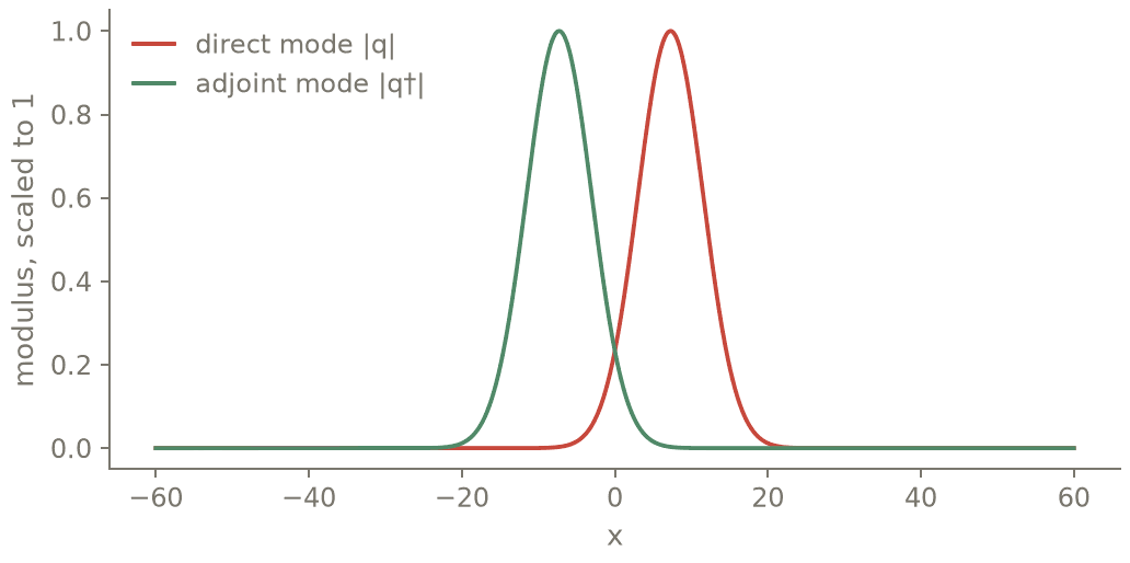
The direct and adjoint global modes of the Ginzburg-Landau model of the page. Advection pushes the direct mode downstream and the adjoint upstream: the operator is far from normal.

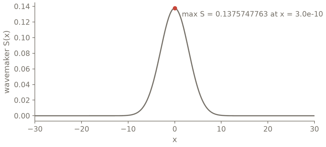
The wavemaker S(x) = |q†(x)| |q(x)|, where the overlap of the two modes is largest: the region where a local change of the model moves the eigenvalue most. The maximum matches Chomaz’s closed form.

Data: DMD in the exact norm

Grid values on Gauss nodes with Fejér weights: the quadrature is exact for the resolved field, so the data norm is the energy norm of the model (EᴴWE = 2I).

# The same model, smaller and more damped (mu_c = -0.2), in energy-orthonormal coordinates.
small = linear_ginzburg_landau(nu=NU, gamma=GAMMA, mu=-0.2 + MU_2 * Y ** 2 / 2, bounds=(-20, 20))
ss = state_space(small.discretize(32), infinite_tol=1e-10)
grid = Grid([Chebyshev(-20.0, 20.0, 64)])                 # values on 64 Gauss nodes
t_nodes = (2 * grid.axes[0].nodes() + 0.0) / 40.0
E = np.polynomial.chebyshev.chebvander(t_nodes, 31) @ ss.to_state      # q -> grid values
ip = DataInnerProduct.from_grid(grid, components=["q"], weights={"q": 1.0})

# (1) DMD of a free transient started in the span of the 4 least stable global modes
dt = 0.5
lam, V = np.linalg.eig(ss.A)
lead4 = np.argsort(-lam.real)[:4]
q0 = V[:, lead4] @ np.array([1.0, 0.5j, 0.3, 0.2 - 0.1j])
Phi = sla.expm(ss.A * dt)
X = E @ np.stack([np.linalg.matrix_power(Phi, j) @ q0 for j in range(40)], axis=1)
r = dmd(X, dt=dt, rank=4, inner_product=ip, amplitudes="optimal")
print(r.explain())

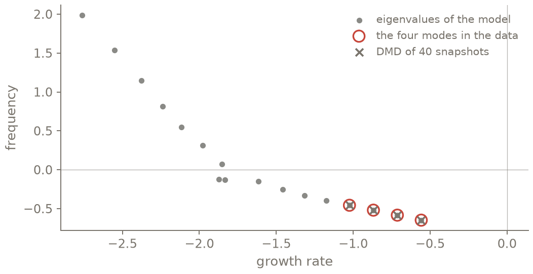
Dynamic mode decomposition of a transient made of four global modes: the DMD eigenvalues (crosses) land on the model’s (red circles) to 10⁻⁹, from the snapshots alone.

Checks

S0 = abs(exact.chi) / np.sqrt(np.pi)                      # Chomaz (2005): S_0(0) = |chi|/sqrt(pi)
assert abs(s_star - S0) < 1e-9 * S0 and abs(x_star) < 1e-4
assert abs(dmu2 - 1 / (4 * exact.chi ** 2)) < 1e-9 * abs(dmu2)
for mu in lam[lead4]:
    assert np.min(np.abs(r.omega - mu)) < 1e-9, (mu, r.omega)
print("OK: wavemaker and d lambda/d mu_2 match the closed forms; DMD finds the four least stable "
      "eigenvalues")

Output

# t13_sensitivity_data: PASS (exit 0) in 34.5 s | 2026-10-20 | script sha256 886d2f1f7f80650b
Ginzburg-Landau (whole line) mode n = 0: λ = -0.0176886987015018-0.647820287354721j, χ = 0.239159529837+0.0475717882612j (Re χ² > 0); ν = (2+0.4j), γ = (1-1j), μ_c = 0.34, μ₂ = -0.01. Closed-form direct/adjoint modes, wavemaker, gradient w.r.t. μ(x) and dλ/d(ν, μ_c, μ₂) (Chomaz 2005; Bagheri et al. 2009).
ModePair of 'linear Ginzburg-Landau: nu = (2+0.4j), gamma = (1-1j), mu = 0.34 - 0.005*y**2' (Chebyshev N = 140): σ = -0.0176886987015045-0.647820287354706j; pencil residuals right 1.4e-16, left 1.1e-16; physical adjoint = continuous adjoint (eigenvalue -0.0176886987015126+0.647820287354736j, residual 2.8e-17); product ⟨a,b⟩ = Σ w_i ∫ ā_i b_i dy, w = {'q': 1.0}; normalization ⟨u,u⟩ = 1, ⟨u†,u⟩ = 1; κ = 19.1473. nearest other finite eigenvalue at distance 1.682e-01
wavemaker maximum S = 0.137574776291 at x = 3.98e-11
d lambda/d mu_2 = 3.884434935074-1.608985632263j (density)  3.884434935072-1.608985632266j (pencil)
DMD (exact, rank 4, Δt = 0.5, amplitudes 'optimal', quadrature product): ω = -0.5576897846-0.6478195408j (|b| 1.41, res 1.2e-14); ω = -0.7130915004-0.5834606995j (|b| 0.707, res 8.2e-14); ω = -0.8686490565-0.5192373431j (|b| 0.424, res 2.4e-13); ω = -1.024295602-0.4562651356j (|b| 0.316, res 1.4e-13); misfit 3.5e-14; principal log (|Im ω| < π/Δt = 6.28319). 
OK: wavemaker and d lambda/d mu_2 match the closed forms; DMD finds the four least stable eigenvalues