15. Covariant Lyapunov vectors of Kuramoto–Sivashinsky: tangencies and the physical modes

The Lyapunov exponents say how fast perturbations grow; the covariant Lyapunov vectors say in which directions, and the angles between them say whether the tangent space splits cleanly. In the Kuramoto–Sivashinsky equation on \(L = 22\) the first eight vectors keep touching each other while the rest stay apart: eight “physical” modes carry the dynamics.

Goal. Compute the twelve leading exponents and covariant vectors of KS \(L = 22\) from a native model with sim.lyapunov, check their covariance, and count the entangled modes from the domination of the Oseledets splitting. Expected. Cvitanović, Davidchack & Siminos (2010, p. 12): \((0.048, 0, 0, -0.003, -0.189, -0.256, -0.290, -0.310, -1.963, -1.967, \dots)\) in the zero-mean subspace; Ding, Chaté, Cvitanović, Siminos & Takeuchi (2016): eight physical modes. Time: about two minutes on one CPU core. Script: t15_ks_covariant.py · Tests behind it: tests/chaos/.

The model and four starts

L = 22.0
m = cn.Model(cn.Box(x=cn.periodic(L)), name="Kuramoto-Sivashinsky L=22")
m.scalar("u")
m.equations("dt(u) + lap(u) + lap(lap(u)) = -u*dx(u)")
sim = m.simulate(N=32, scheme="RK443", dt=0.05)   # 32 modes, as in the references


def start(c):
    """A smooth zero-mean initial state from four random modes."""
    return {"u": lambda x: 0.3 * sum(c[j, 0] * np.cos(2 * np.pi * (j + 1) * x / L)
                                     + c[j, 1] * np.sin(2 * np.pi * (j + 1) * x / L)
                                     for j in range(4))}


rng = np.random.default_rng(7)
starts = [start(rng.standard_normal((4, 2))) for _ in range(4)]

The starts are sim.initial keyword dicts: each becomes one trajectory of the same batch, and the simulation’s own state is left as it was.

Exponents and covariant vectors

res = sim.lyapunov(12, transient=100.0, align=50.0, T=200.0, reortho_every=10,
                   inner="euclidean", n_blocks=4, seed=1, starts=starts, zero_mean="u",
                   covariant=True, clv_window=40.0, clv_backward=40.0, clv_checkpoints=8)
print(res.explain())

Every length is a time of the problem: transient (trajectory only), align (the tangent vectors align with the Oseledets directions), T (averaging), clv_window and clv_backward (the covariant vectors are computed over a window that ends 40 time units before the end, the time the backward iteration needs to converge). Each must be a whole number of steps or of intervals reortho_every * dt; nothing is rounded. zero_mean="u" keeps the tangent vectors in the invariant zero-mean subspace, as in the references. clv_checkpoints=8 stores 8 checkpoints instead of every interval and recomputes them once; explain() gives the memory used, the difference between recomputed and stored factors (zero), the backward convergence (the vectors obtained from two independent random starts of the backward iteration, compared: small except inside nearly degenerate pairs such as the two zero exponents, which converge slowly) and the covariance residual: each vector advanced by the exact tangent over one interval must be parallel to the vector there, to its rounding floor.

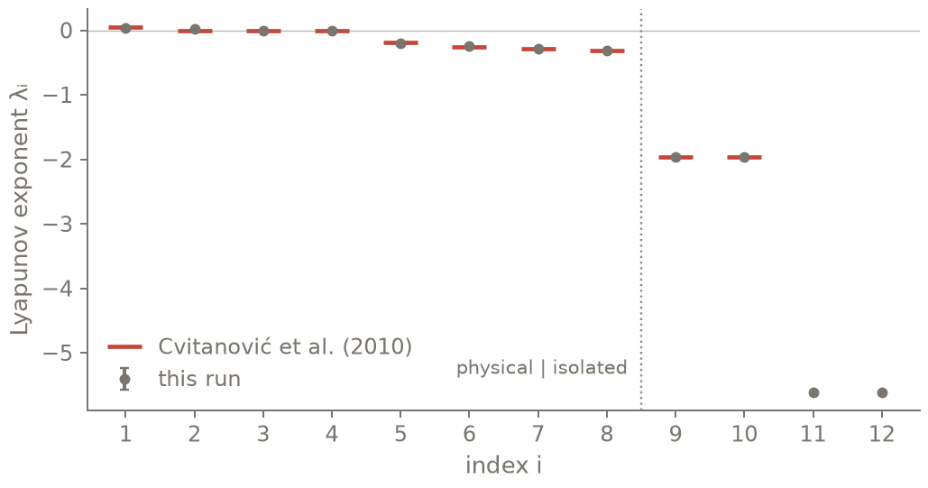
The twelve leading exponents of Kuramoto-Sivashinsky at L = 22, with their standard errors, on the published values. The first eight are the physical modes.

Tangencies and domination

dom = res.domination(tau=5.0)
print(dom.explain())
theta8 = res.angles(8)                     # span(gamma_1..gamma_8) vs the rest, every sample
theta4 = res.angles(4)
print(f"smallest angle at the split 8 | 9: {theta8.min():.3f} rad; at 4 | 5: "
      f"{theta4.min():.4f} rad ({np.mean(theta4 < 0.1):.0%} of the samples below 0.1 rad)")

domination(tau) compares the local growth rates of the vectors over windows of length \(\tau\): whenever \(\Lambda_i < \Lambda_j\) for \(i < j\) the splitting is not dominated there. Modes joined by such violations form clusters; the leading cluster is the set of physical modes. The principal angles tell the same story: the split \(8 \mid 9\) keeps a finite angle, the split \(4 \mid 5\) inside the physical block has near-tangencies.

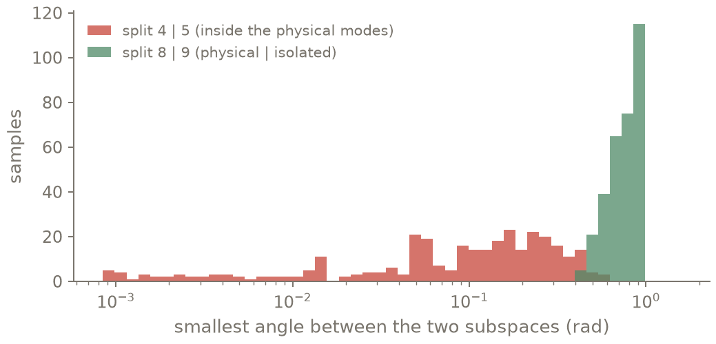
Angles between the span of the first j covariant vectors and the rest, at every sample. Inside the physical modes (j = 4) near-tangencies are frequent; at j = 8 the split never closes.

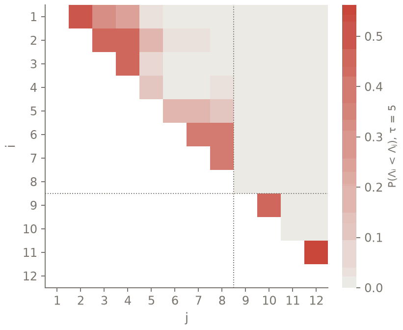
Domination of Oseledets splitting: how often the local exponent i falls below j over windows of 5 time units. Violations stay among the first eight modes: they form one entangled block.

Check

cds = np.array([0.048, 0.0, 0.0, -0.003, -0.189, -0.256, -0.290, -0.310, -1.963, -1.967])
dev = np.abs(res.exponents[:10] - cds)
assert np.all(dev < 4 * res.stderr[:10] + 0.01), (res.exponents[:10], res.stderr[:10])
# J gamma_i(t) is parallel to gamma_i(t + dt_interval), to the rounding floor of each vector
assert np.all(res.clv_covariance_residual < 100 * res.clv_covariance_floor)
assert dom.n_physical == 8 and dom.violation(8) == 0.0
assert res.clv_split_convergence[7] < 1e-6            # the split 8 | 9 itself has converged
assert theta8.min() > 10 * theta4.min()               # isolated split versus tangencies
print("checks passed: exponents within their errors of CDS 2010, eight physical modes")

Output (as executed)

# t15_ks_covariant: PASS (exit 0) in 52.4 s | 2026-10-20 | script sha256 77224d7831ae3936
Lyapunov spectrum of the discrete map (RK443, dt = 0.05, backend = cpu): 12 vector(s), 4 trajectory(ies)
  transient 2000 steps, tangent transient 1000 steps, average over T = 200 per trajectory (400 QR every 10 steps = 0.5)
  inner product: Euclidean on the coefficient vector; projection: zero mean: the wavenumber-zero coefficient of u set to 0 in every tangent vector (1 component(s) of the state vector); seed 1
  error: standard error of 16 block means (4 per trajectory), max |lag-1 corr| = 0.57
  λ1   = +0.04069 ± 0.00724   (CLV growth +0.03296)
  λ2   = +0.01555 ± 0.00704   (CLV growth -0.00449)
  λ3   = -0.00720 ± 0.00457   (CLV growth -0.01593)
  λ4   = -0.00854 ± 0.00688   (CLV growth -0.03638)
  λ5   = -0.20116 ± 0.01460   (CLV growth -0.19187)
  λ6   = -0.23875 ± 0.00953   (CLV growth -0.29066)
  λ7   = -0.29046 ± 0.01057   (CLV growth -0.30125)
  λ8   = -0.31677 ± 0.00836   (CLV growth -0.31087)
  λ9   = -1.96531 ± 0.00489   (CLV growth -1.95621)
  λ10  = -1.96288 ± 0.00444   (CLV growth -1.95919)
  λ11  = -5.60754 ± 0.00212   (CLV growth -5.60539)
  λ12  = -5.60776 ± 0.00200   (CLV growth -5.60469)
  sum = -16.15014
  Kaplan–Yorke dimension = 4.2013 ± 0.0895
  covariant vectors (Ginelli et al. 2007): 80 kept time(s) x 4 trajectory(ies), window 80 interval(s) after a backward transient of 80, kept every 1
  memory: checkpointed: 8 checkpoint(s) (Q, X) every 20 interval(s), 160 R matrices, one segment of at most 20 Q_j recomputed at a time: 1.05 MiB instead of 2.67 MiB, for one extra forward pass over the 160 stored intervals
  recomputed R vs stored R: max relative difference 0.00e+00
  backward convergence (sine of the angle between the CLVs of two independent random backward starts): max 1.00e+00 (worst vector 10); slow for nearly equal exponents (rate λ_i-1 - λ_i): lengthen clv_backward if it matters
  subspace convergence per split j (span(γ_j+1..γ_k), two starts, largest sine; rate λ_j - λ_j+1): 1.0e+00, 1.0e+00, 1.0e+00, 2.3e-02, 7.0e-01, 9.9e-01, 1.0e+00, 3.3e-15, 1.0e+00, 3.9e-15, 8.6e-01
  covariance residual (sine of the angle between J γ_i(t_j) and γ_i(t_j+1) over one interval; consistency of the stored factors with the tangent): max 6.23e-15 (vector 12); largest ratio to its rounding floor eps exp((λ_1 - λ_i) Δt): 4.34 (vector 7)
  smallest principal angle between span(γ_1..γ_j) and the rest, j = 1..11: 0.0022, 0.000415, 8.75e-05, 0.000844, 0.00388, 0.011, 0.069, 0.448, 0.143, 0.94, 0.145 rad
  note: 12 of 31 exponents computed: sum and Kaplan–Yorke use these only
  note: native: sim.lyapunov on 'Kuramoto-Sivashinsky L=22' (transient 100, align 50, T 200 per trajectory, CLV window 40 ending 40 before the end); the simulation's own state is not advanced
Domination of the Oseledets splitting at tau = 5: 32 samples (windows x trajectories), 12 covariant vectors
  violation fraction across each split j | j+1 (largest nu_ij, i <= j < l): 1:0.5, 2:0.438, 3:0.469, 4:0.188, 5:0.188, 6:0.375, 7:0.375, 8:0, 9:0.438, 10:0, 11:0.562
  clusters of entangled modes (any observed violation joins them): 1-8, 9-10, 11-12
  physical modes (leading entangled cluster): 8; the split after it has violation 0 and smallest principal angle 0.448 rad (its subspaces converged to 3.3e-15)
  a violation fraction is a sample estimate: 0 means none observed in 32 samples; modes near k may entangle with modes not computed
smallest angle at the split 8 | 9: 0.448 rad; at 4 | 5: 0.0008 rad (47% of the samples below 0.1 rad)
checks passed: exponents within their errors of CDS 2010, eight physical modes

Going further

• The same call on the GPU: m.simulate(..., backend="cuda"), nothing else changes (not yet verified against the CPU on GPU hardware: experimental until tests/model/test_particles_gpu.py has run).