0. Getting started: convection between two plates

One problem from beginning to end: a layer of fluid heated from below. You write its equations as on paper, ask whether the fluid at rest is stable, find where convection starts (the published value to \(2\times10^{-4}\) in \(Ra_c\) and \(7\times10^{-4}\) in \(k_c\)), then simulate the rolls that appear above onset and measure the heat they carry. New to Conatus? The ten-minute Getting started in ten minutes comes before this one.

Expected. Onset at \(Ra_c = 1707.762\), \(k_c = 3.117\) between rigid plates (Reid & Harris 1958; Chandrasekhar 1961); the script finds \(Ra_c = 1707.7618\) (absolute difference \(2\times10^{-4}\), relative \(10^{-7}\): the published value is rounded) and \(k_c = 3.11632\) (difference \(7\times10^{-4}\), relative \(2\times10^{-4}\): the tabulated 3.117 differs in its fourth digit) and checks both to \(10^{-3}\); the simulation grows at the eigenvalue’s rate; the saturated rolls carry the same heat through both plates and across the layer. Time: about two minutes of CPU (136 s on a cluster CPU node). Needs: the tutorials extra (pip install "conatus[tutorials]", Installation). Script: t00_getting_started.py.

The model

In thermal-diffusion units, \(z \in [-1/2, 1/2]\), rigid plates at fixed temperatures:

\[ \partial_t \mathbf{u} + \mathbf{u}\cdot\nabla\mathbf{u} = -\nabla p + Pr\,\nabla^2 \mathbf{u} + Pr\,Ra\,T\,\mathbf{e}_z,\qquad \nabla\cdot\mathbf{u} = 0,\qquad \partial_t T + \mathbf{u}\cdot\nabla T = \nabla^2 T, \]

with \(\mathbf{u} = 0\) and \(T = \pm 1/2\) on the plates \(z = \mp 1/2\).

import numpy as np

import conatus as cn
from conatus.expert import critical

def convection(Ra):
    """Rayleigh-Benard convection between two plates; one roll pair fits the box of length 2."""
    box = cn.Box(x=cn.periodic(2.0), z=cn.walls(-0.5, 0.5))   # x periodic, plates at z = -1/2, 1/2
    m = cn.Model(box, name="Rayleigh-Benard", Ra=Ra, Pr=1)
    m.velocity("u"), m.pressure("p"), m.scalar("T")
    m.equations("""
        momentum:   dt(u) + grad(p) - Pr*lap(u) = Pr*Ra*T*ez - u·grad(u)
        continuity: div(u) = 0
        heat:       dt(T) - lap(T) = -u·grad(T)
    """)
    m.at("bottom", u=0, T=+0.5)                # hot plate below, no slip
    m.at("top", u=0, T=-0.5)                   # cold plate above, no slip
    return m


m = convection(Ra=2500)
print(m.explain())

The domain names its boundaries (bottom, top); conditions are stated where they hold. There is no basis to choose and nothing to say about how the conditions are imposed: m.explain() sums up the implicit–explicit split, the conditions by wall, the pressure gauge and the dealiasing, all placed by fixed rules (see the output at the end of the page); m.explain(full=True) lists every decision, tau by tau and term by term.

Is the fluid at rest stable?

growth = {}
for Ra in (1500, 2500):
    lin = convection(Ra).linearize(about={"u": 0, "T": lambda z: -z})   # fluid at rest, T = -z
    modes = lin.eigenvalues(N=24, k=np.pi)     # 24 Chebyshev modes across, roll wavenumber pi
    growth[Ra] = modes.values.real.max()
    print(f"Ra = {Ra}: largest growth rate {growth[Ra]:+.6f}")

linearize derives the linear equations about the conduction state \(T = -z\); eigenvalues solves them for the roll \(k = \pi\) with the resolution you choose. At \(Ra = 1500\) every disturbance decays; at \(Ra = 2500\) one grows.

Where convection starts

A disturbance \(\propto e^{ikx + st}\) obeys two ordinary differential equations in \(z\), written here as a model on a line with the eigenvalue \(s\) declared:

onset = cn.Model(cn.Box(z=cn.walls(-0.5, 0.5)), name="convection onset", Ra=1700.0, k=3.1, Pr=1)
onset.scalar("w"), onset.scalar("theta")      # w(z), theta(z) times exp(i k x + s t)
onset.eigenvalue("s", growth="real")
onset.define("L(f) = dz(dz(f)) - k**2*f")     # the Laplacian of one Fourier mode
onset.equations("""
    momentum: s*L(w) = Pr*L(L(w)) - Pr*Ra*k**2*theta
    heat:     s*theta = w + L(theta)
""")
onset.at("walls", "w = 0", "dz(w) = 0", "theta = 0")
# drift=48: a mode counts only if it is found again at 48 modes (spurious tau modes are not)
P = onset.parametric(N=32, over=("Ra", "k"), drift=48, drift_tol=1e-6)
crit = critical(P, "Ra", bracket=(1500, 2000), over={"k": (2.8, 3.4)}, xtol=1e-9)
print(f"Ra_c = {crit.value:.4f}   k_c = {crit.over['k']:.5f}")

parametric keeps \(Ra\) and \(k\) as live parameters; critical finds the neutral \(Ra\) and minimises it over \(k\). drift=48 sets aside the spurious modes of the boundary treatment: a mode is kept only if the same pencil at 48 modes has it too, within drift_tol (a physical mode is resolved and does not move; a spurious one jumps). The growth of \(s\) is its real part, read off its name and printed by crit.explain().

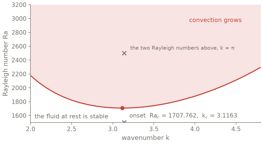
Growth rate of the least stable mode over a grid of (k, Ra), from the parametric pencil of the onset block. The red line is where it vanishes; its minimum is the critical point the script finds, Ra_c = 1707.762 at k_c = 3.1163.

Simulate above onset

sim = m.simulate(N=(32, 24), scheme="RK443", dt=5e-4)
sim.initial(T=lambda x, z: -z + 1e-6 * np.cos(np.pi * x) * np.cos(np.pi * z))


def roll_amplitude(sim):
    """Largest departure of T from its horizontal mean: the size of the rolls."""
    T = sim.grid("T")
    return np.abs(T - T.mean(axis=0)).max()


sim.run(until=0.3)
a1, t1 = roll_amplitude(sim), sim.t
sim.run(until=0.8)
a2, t2 = roll_amplitude(sim), sim.t
sigma = np.log(a2 / a1) / (t2 - t1)
print(f"measured growth rate {sigma:.6f}   eigenvalue {growth[2500]:.6f}")

The simulation and the eigenvalue problem come from the same model; while the disturbance is small they agree.

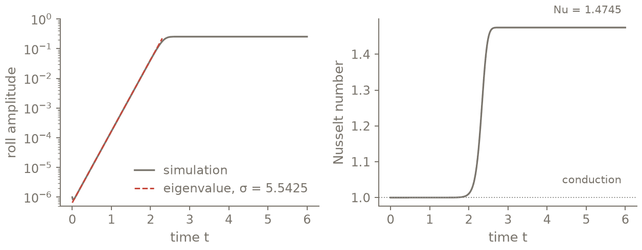
The simulation of the page. Left: the rolls grow at the rate of the eigenvalue (dashed) until the nonlinear terms stop them. Right: the heat carried across the layer, in units of conduction, settles to a steady value.

Steady rolls and the heat they carry

from conatus.diagnostics import Chebyshev, Grid, Periodic

grid = Grid([Periodic(2.0, 32), Chebyshev(-0.5, 0.5, 24)])   # the simulation's grid points
profile = Grid([Chebyshev(-0.5, 0.5, 24)])                    # functions of z alone


def nusselt(sim):
    """Heat carried across the layer in units of conduction, measured three ways."""
    w, T = sim.grid("u")[1], sim.grid("T")
    layer = 1 + float(grid.mean(w * T))       # conduction + convection, averaged over the layer
    dTdz = profile.cheb_coeffs(profile.d(T.mean(axis=0), 0), 0)
    bottom = -np.polynomial.chebyshev.chebval(-1.0, dTdz)    # conduction through each plate
    top = -np.polynomial.chebyshev.chebval(+1.0, dTdz)
    return layer, bottom, top

with cn.runs.track("rb_Ra2500", tags=["getting-started"], root="runs") as run:
    sim.solver.run(round((6.0 - sim.t) / sim.dt), record=run)     # on to t = 6
    Nu_layer, Nu_bottom, Nu_top = nusselt(sim)
    run.result(Nu=Nu_layer)
print(f"t = {sim.t:.1f}: Nu = {Nu_layer:.6f} (layer)  {Nu_bottom:.6f} (bottom plate)  "
      f"{Nu_top:.6f} (top plate)")
print(run.explain().splitlines()[0])
print(sim.methods().explain())

In a steady state the heat entering through the hot plate crosses every level and leaves through the cold one: the three values of \(Nu\) agree.

The checks

RA_C, K_C = 1707.762, 3.117                    # Reid & Harris (1958); Chandrasekhar (1961)
assert abs(crit.value - RA_C) < 1e-3 and abs(crit.over["k"] - K_C) < 1e-3, crit
assert growth[1500] < 0 < growth[2500], growth
assert abs(sigma - growth[2500]) < 1e-5, (sigma, growth[2500])
assert Nu_layer > 1 and abs(Nu_bottom - Nu_layer) < 1e-3 * Nu_layer \
    and abs(Nu_top - Nu_layer) < 1e-3 * Nu_layer, (Nu_layer, Nu_bottom, Nu_top)
print("OK: onset at Reid & Harris' Ra_c and k_c; the simulation grows at the eigenvalue's rate "
      "and saturates into rolls carrying the same heat through both plates")

Output

# t00_getting_started: PASS (exit 0) in 138.6 s | 2026-10-20 | script sha256 f95681b44467db9d
Model 'Rayleigh-Benard': Box(x=periodic((0, 2)), z=walls(-0.5, 0.5)) (Cartesian box)
Unknowns: u (velocity), p (pressure), T (scalar); parameters: Ra = 2500, Pr = 1
Equations as written:
  momentum: dt(u) + grad(p) - Pr*lap(u) = Pr*Ra*T*ez - u·grad(u)
  continuity: div(u) = 0
  heat: dt(T) - lap(T) = -u·grad(T)
Problem: IVP (a time derivative dt() appears)
Time stepping: 7 linear term(s) implicit; nonlinear terms explicit (momentum, heat)
Boundary conditions: bottom: u = 0, T = 0.5; top: u = 0, T = -0.5 (tau method, placed automatically)
Gauge: the mean of p is fixed (integ(p) = 0)
Dealiasing: x: 3/2, z: 3/2 (declared default for products of degree 2)
Resolution: not chosen yet (simulate/eigenvalues/discretize(N=...))
(every decision, tau by tau and term by term: m.explain(full=True))
Ra = 1500: largest growth rate -1.637012
Ra = 2500: largest growth rate +5.542506
Ra_c = 1707.7618   k_c = 3.11632
measured growth rate 5.542508   eigenvalue 5.542506
t = 6.0: Nu = 1.474455 (layer)  1.474455 (bottom plate)  1.474455 (top plate)
Run (rb_Ra2500): state completed, status provisional, 87.8 s
Methods paragraph generated from the plan (edit before publishing):

The IVP 'Rayleigh-Benard' for (u, p, T) was solved with Conatus. The domain is discretized as follows: x ∈ [0, 2) is periodic and expanded in a real (cosine/sine) Fourier series of 32 modes; z ∈ [-0.5, 0.5] is expanded in 24 Chebyshev polynomials of the first kind. Derivatives, basis conversions and multiplications by non-constant coefficients use the sparse, banded ultraspherical operators of Olver & Townsend, and boundary conditions are imposed with the generalized tau method (4 tau variable(s), each entering through a lift polynomial), following Burns et al. The Fourier directions decouple, giving 16 independent systems, one per wavenumber. Nonlinear terms are evaluated pseudospectrally with dealiasing factors 3/2 in x, 3/2 in z. The structural rank of every system was checked before factorization. Time integration uses the third-order, four-stage IMEX Runge–Kutta scheme (4,4,3) of Ascher, Ruuth & Spiteri, whose implicit diagonal is constant so that a single factorization serves all stages, with a constant step Δt = 0.0005. The implicit systems are solved by banded LU factorization with a low-rank (Woodbury) correction for the tau rows, batched over wavenumbers on CPU, in float64 arithmetic. The equations were declared in the native layer of Conatus as written on paper; the implicit-explicit split, the 4 tau term(s) (each in the equation where its unknown has its highest wall-normal order) and the pressure gauge and its integral constraint were placed by fixed, declared rules (listed by explain()). The dealiasing factor 3/2 is the declared default of the native layer ((p+1)/2 for the highest polynomial degree p = 2 of the equations in the unknowns and given fields, at least 3/2).

Citations: olver2013, burns2020, ascher1997
Facts used: kind=IVP, groups=16, N_x=32, N_z=24, zbasis=Chebyshev, taus=4, dealias={'x': 1.5, 'z': 1.5}, scheme=RK443, dt=0.0005, backend=cpu, native=True, dealias_default=True
OK: onset at Reid & Harris' Ra_c and k_c; the simulation grows at the eigenvalue's rate and saturates into rolls carrying the same heat through both plates

Next: tutorials 1 to 14, starting with 1. A first eigenvalue problem: Orr–Sommerfeld.