8. Polar geometry: a drum, a pipe, two rotating cylinders

The same workflow runs on the disk, the annulus and the cylinder, on regular bases, with nothing divided by \(r\).

Goal. Solve three classical eigenvalue problems in polar and cylindrical geometry: the modes of a vibrating drum, written as a native model on cn.Disk; the linear stability of Hagen–Poiseuille flow in a pipe; and the onset of Taylor vortices between rotating cylinders. The last two come from the library of ready problems (cn.problems). Expected. Drum: eigenvalues \(-j_{m,n}^2\), the squared zeros of the Bessel functions (closed form). Pipe, \(R = 1000\): rightmost eigenvalues of \((m, k) = (1, 1)\) and \((1, 0)\) to 10 decimals (Meseguer & Trefethen 2003, J. Comput. Phys. 186, Table 1). Taylor–Couette, radius ratio \(\eta = 0.5\), outer cylinder at rest: \(Re_c = 68.19\) at \(k_c = 3.16\) (Recktenwald, Lücke & Müller 1993, Phys. Rev. E 48, 4444, Table I). Time: under a minute on one CPU core. Script: t08_polar.py · Tests behind it: tests/polar/, tests/problems/test_problems_cylinders.py (also against Dedalus to \(10^{-13}\)).

Regular bases, nothing divided by r

On the disk each component is expanded in a regular (Zernike-type) basis \(\rho^{|m|}\,P_n^{(a,|m|)}(2\rho^2 - 1)\), vectors are stored in spin components \(u_\pm = u_r \pm i u_\varphi\) (regular as \(\rho^{|m\pm1|}\)), and every operator is a sparse map between these bases (Vasil et al. 2016). There is no axis condition to impose and no \(1/(r + \varepsilon)\): regularity at \(r = 0\) is built in. You name the geometry and its wall; explain() prints the bases it chose.

import numpy as np
from scipy.optimize import brentq
from scipy.special import jn_zeros

import conatus as cn
from conatus.expert import eigenvalues

A vibrating drum

drum = cn.Model(cn.Disk(radius=1.0), name="vibrating drum")
drum.scalar("T")
drum.eigenvalue("s", growth="real")
drum.equations("s*T = lap(T)")
drum.at("wall", T=0)
print(drum.explain())
plan = drum.discretize(N=(8, 32))                   # (phi, r): one group per azimuthal number m
drum_modes = {}
for g in plan.groups[:3]:                           # m = 0, 1, 2
    res = eigenvalues(plan, g)
    drum_modes[g.m] = np.sort(res.values.real)[::-1][:3]
    print(f"m = {g.m}: s = {np.round(drum_modes[g.m], 8)}  backward residual "
          f"{res.residuals.max():.1e}")

• cn.Disk(radius=1.0) has one boundary, wall. The model declares an eigenvalue s and the equation \(sT = \nabla^2 T\); the condition \(T = 0\) is given by name. The tau term is placed by the rule of the disk (lifted in the derivative basis), and explain() says so.

• The plan has one block per azimuthal number \(m\). The expert function eigenvalues(plan, group) solves one block; the native drum.eigenvalues(N, m=0) solves the block \(m = 0\) (m= names the block; without it v0.1 solves the first block and says so in a DeprecationWarning).

• The exact answer is \(s = -j_{m,n}^2\): separation of variables gives \(J_m(\sqrt{-s}\,r)\), and the wall condition picks the zeros \(j_{m,n}\) of \(J_m\).

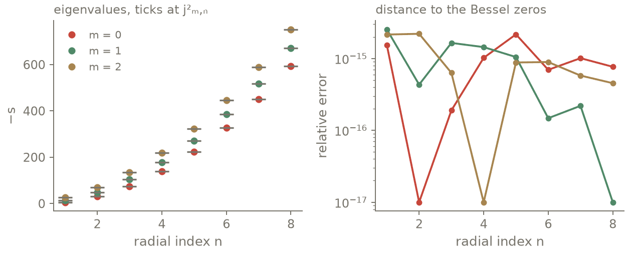
The vibrating drum at N = 32 radial modes: the eight slowest modes of each azimuthal group against the closed form −j²ₘ,ₙ. The first ones agree to rounding; the error grows with n as the modes become finer than the grid.

Hagen–Poiseuille

hp = cn.problems.pipe_evp(N=32, Re=1000.0, m=1, k=1.0)   # ready problem: equations and walls
print(hp.problem.name, "|", hp.notes.strip())   # hp.explain(): equations, bases, reference
plan = cn.discretize(hp.problem, ncc=hp.ncc)
res = eigenvalues(plan, plan.group(1, 1.0))         # one group per (m, k_z)
top = res.values[np.argsort(-res.values.real)[:3]]
print("rightmost eigenvalues (m, k) = (1, 1):", np.round(top, 10))
print(f"max backward residual {res.residuals.max():.1e}")
s10 = eigenvalues(plan, plan.group(1, 0.0)).values  # k = 0 is also a group of this plan
s10 = s10[np.argmax(s10.real)]

• cn.problems.pipe_evp returns an ordinary problem: the linearised Navier–Stokes equations about \(U_0 = (1 - r^2)\,\mathbf{e}_z\), no slip at \(r = 1\), with its validation reference. hp.explain() prints the equations, bases and conditions; open the function to read or copy it.

• The plan has one block per \((m, k_z)\): plan.group(1, 1.0); \(k_z = 0\) is a block of the same plan. Each block gets its own rank report before any solve.

• Sign convention: Meseguer & Trefethen’s Table 1 lists \(\operatorname{Im}\lambda\) with the opposite sign to the one implied by their own eq. (15) and \(V_t = \mathcal{L}V\) (the centre mode advected by \(W \approx 1\) must have \(\operatorname{Im}\lambda \approx -k\)); Dedalus agrees with Conatus. The comparison is made with the conjugate, and that is written in the check.

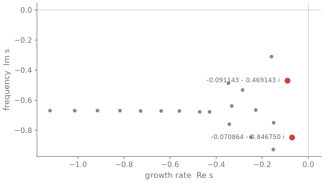
Hagen-Poiseuille flow, R = 1000, (m, k) = (1, 1): the spectrum of the pipe block. All modes decay; the two least stable (red) are the centre and wall modes of Meseguer and Trefethen.

Taylor–Couette

def couette_growth(Re, k, N=24):
    """Largest growth rate of axisymmetric (m = 0) perturbations with axial wavenumber k."""
    tc = cn.problems.taylor_couette_evp(N=N, Re=Re, eta=0.5, mu=0.0, m=0, k=k)
    plan = cn.discretize(tc.problem, ncc=tc.ncc)
    return eigenvalues(plan, plan.group(0, k)).values.real.max()


Re_c = {k: brentq(lambda Re, k=k: couette_growth(Re, k), 60.0, 80.0, xtol=1e-6) for k in (3.10, 3.16, 3.22)}
kc = min(Re_c, key=Re_c.get)
print("neutral Re(k):", {k: round(v, 4) for k, v in Re_c.items()})

Units: gap \(d = r_o - r_i = 1\), inner wall speed \(\Omega_i r_i = 1\), \(Re = \Omega_i r_i d/\nu\). The base flow is circular Couette flow \(V(r) = Ar + B/r\). For each \(k\) the neutral Reynolds number (largest growth rate \(= 0\)) is found by Brent’s method on the dense spectrum of the axisymmetric block \((m, k_z) = (0, k)\); the minimum over three wavenumbers brackets \(k_c\).

Check against the references

The drum eigenvalues equal \(-j_{m,n}^2\) to \(10^{-12}\) relative. The pipe eigenvalues match Meseguer & Trefethen’s to the 10 published decimals. The Taylor–Couette threshold \(Re_c = 68.1863\), converged in \(N\), agrees with the published \(68.19\) to its 4 digits.

for m in (0, 1, 2):                                 # -j_{m,n}^2, closed form
    assert np.allclose(drum_modes[m], -jn_zeros(m, 3) ** 2, rtol=1e-12, atol=0), m
MT_CENTRE, MT_WALL, MT_K0 = -0.0708640053 + 0.8467498288j, -0.0911426036 + 0.4691428789j, -0.0146819706
for ref in (MT_CENTRE, MT_WALL):                    # Table 1 lists the conjugate (see the page)
    assert np.min(np.abs(res.values - np.conj(ref))) < 1e-10
assert abs(s10 - MT_K0) < 1e-10 and res.residuals.max() < 1e-13
assert kc == 3.16 and abs(Re_c[kc] - 68.19) < 0.01   # published to 4 digits
print(f"OK: drum = Bessel zeros; pipe eigenvalues to 1e-10 of Meseguer & Trefethen; "
      f"Re_c(3.16) = {Re_c[kc]:.4f}")

Output (as executed)

# t08_polar: PASS (exit 0) in 33.7 s | 2026-10-20 | script sha256 b188c872c8126df9
Model 'vibrating drum': Disk(radius=1) (disk)
Unknowns: T (scalar)
Eigenvalue: s; growth = Re s, declared with the eigenvalue s
Equations as written:
  eq0: s*T = lap(T)
Problem: EVP (eigenvalue s declared)
Boundary conditions: wall: T = 0 (tau method, placed automatically)
Dealiasing: phi: 3/2, r: 3/2 (declared default for products of degree 1)
Resolution: not chosen yet (simulate/eigenvalues/discretize(N=...))
(every decision, tau by tau and term by term: m.explain(full=True))
m = 0: s = [ -5.78318596 -30.47126234 -74.88700679]  backward residual 7.8e-15
m = 1: s = [ -14.68197064  -49.21845632 -103.4994539 ]  backward residual 3.8e-15
m = 2: s = [ -26.37461643  -70.84999892 -135.02070887]  backward residual 2.1e-15
Hagen-Poiseuille stability | Use plan.group(1, 1.0). Eigenvalue s = sigma + i omega.
rightmost eigenvalues (m, k) = (1, 1): [-0.07086401-0.84674983j -0.0911426 -0.46914288j -0.15121606-0.74819401j]
max backward residual 1.3e-15
neutral Re(k): {3.1: 68.2054, 3.16: 68.1863, 3.22: 68.2021}
OK: drum = Bessel zeros; pipe eigenvalues to 1e-10 of Meseguer & Trefethen; Re_c(3.16) = 68.1863

Going further

• Time integration on the disk, annulus, sphere, ball and shell uses the same native calls (m.simulate(...)); see Geometries.

• The ready problems cn.problems.pipe, taylor_couette and rotating_shell_convection give the nonlinear versions of these flows.