5. Invariant solutions: Kuramoto–Sivashinsky, L = 22

Goal. Find the equilibria, a travelling wave and the shortest pre-periodic orbit of the Kuramoto–Sivashinsky equation on the \(L = 22\) domain by Newton–Krylov–hookstep on the time-stepper’s flow map, with their stability. Expected. Equilibria \(E_1\), \(E_2\) (energies \(0.2609\), \(0.4382\); leading eigenvalues of \(E_1\) \(0.1308 \pm 0.3341i\), \(0.0824 \pm 0.3402i\)), travelling wave \(TW_1\) (\(c = 0.73699\), energy \(0.4649\)): Cvitanović, Davidchack & Siminos (2010), SIAM J. Appl. Dyn. Syst. 9, 1–33, Tables 5.1–5.2 and §5. Pre-periodic orbit \(\overline{pp}_{10.25}\): leading Floquet exponent \(\mu_1 = 0.033209\), \(\theta_1 = 2.0079\) (Ding & Cvitanović 2016, SIAM J. Appl. Dyn. Syst. 15, Table 1). Time: about a minute on one CPU core (the orbit’s dense monodromy dominates). Script: t05_ks_orbits.py · Tests behind it: tests/ecs/.

The system

\[ u_t + u u_x + u_{xx} + u_{xxxx} = 0, \qquad x \in (0, 22) \ \text{periodic}. \]

It is equivariant under translations \(\tau_\ell u(x) = u(x + \ell)\) and the reflection \(R u(x) = -u(-x)\). Invariant solutions come in families: equilibria (\(\Phi_t u = u\)), travelling waves (\(\Phi_t u = \tau_{-ct} u\)), relative periodic orbits (\(\tau_\ell \Phi_T u = u\)) and pre-periodic orbits (\(R\,\Phi_T u = u\)).

The equation, as written

import numpy as np

import conatus as cn
from conatus.expert import (NewtonKrylovHookstep, equilibrium_eigenvalues, find_equilibrium,
                            find_relative_periodic_orbit, find_travelling_wave, floquet_multipliers)

L, N = 22.0, 32
m = cn.Model(cn.Box(x=cn.periodic(L)), name="Kuramoto-Sivashinsky L=22")
u = m.scalar("u")
m.equations("dt(u) + lap(u) + lap(lap(u)) = -u*dx(u)")   # split: linear implicit, u u_x explicit
sim = m.simulate(N=N, scheme="RK443", dt=0.01)
ks = sim.solver                                           # the flow map Phi_T used by every search


def newton(max_it=40):
    """Trust-region Newton--Krylov: the accuracy target tol is required; the algorithm controls
    (GMRES tolerance and budget, trust radii) keep their declared defaults (nk.explain())."""
    return NewtonKrylovHookstep(tol=1e-12, max_iterations=max_it)


def state(u0):
    """Search seed: the state vector of the simulation started from u(x) = u0(x)."""
    sim.initial(u=u0)
    return ks.X.copy()


def sine(n, a):
    """u0 = a sin(2 pi n x / L)."""
    return lambda x: a * np.sin(2 * np.pi * n * x / L)

The model is one line: m.explain() would show the split (the linear terms implicit, \(u u_x\) explicit) and the declared default dealiasing 3/2. The searches never see the equation: they see the flow map \(\Phi_T\) of the simulation’s time stepper (sim.solver, RK443 at \(dt = 0.01\)) and its exact tangent (Jacobian–vector products through the same stepper). Any model with dt() can be searched the same way, within the scope of these finders: one periodic direction (1D problems such as KS; flows with walls use the drivers listed in Invariant solutions). NewtonKrylovHookstep is a trust-region (hookstep) Newton with GMRES: its accuracy target tol is required, its algorithm controls (GMRES tolerance and Krylov budget, trust radii) have declared defaults that nk.explain() prints and marks. state(u0) turns an initial condition written as a function of \(x\) into the state vector the searches start from.

Equilibria and their stability

E1 = find_equilibrium(ks, state(sine(1, 1.0)), newton())
E2 = find_equilibrium(ks, state(sine(2, 1.0)), newton())
ev1 = equilibrium_eigenvalues(ks, E1, n_modes=8, dense_max=500, arnoldi_tol=1e-12)
print(E1.explain())
print(f"E1: energy {E1.energy:.4f}, residual {E1.residual:.1e}; leading eigenvalues",
      np.round(ev1[:4], 4))
print(f"E2: energy {E2.energy:.4f}, residual {E2.residual:.1e}")

The seeds are single sine modes, \(u_0 = \sin(2\pi n x/L)\). A seed that falls back to \(u = 0\) is marked retracted (the trivial-state threshold is declared in explain()), never reported as a new solution. The stability eigenvalues come from the linearised flow at the equilibrium.

A travelling wave

# A seed stored by an earlier search (a draw of four random Fourier modes from which Newton
# converges to the wave; most draws fall back to an equilibrium): the cos and -sin amplitudes of
# modes 1 to 4, written here so that the tutorial does not depend on a random stream.
a = [0.34389095585778406, 0.5568341791702948, -0.9472943734057513, -0.529362057631228,
     -0.349148197714577, -0.9358415262182913, 1.3914943017041073, -0.3967285827537215]
k = 2 * np.pi * np.arange(1, 5) / L
TW1 = find_travelling_wave(ks, state(lambda x: sum(a[2 * i] * np.cos(k[i] * x) - a[2 * i + 1]
                                                   * np.sin(k[i] * x) for i in range(4))),
                           0.737, newton(60))
print(f"TW1: c = {TW1.params['c']:.5f}, energy {TW1.energy:.4f}, residual {TW1.residual:.1e}")

The speed \(c\) is an unknown of the Newton system, with a phase condition that removes the translation degeneracy.

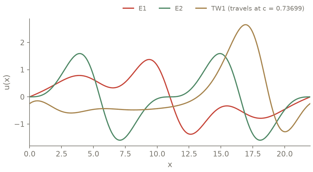
The two equilibria and the travelling wave found by Newton-Krylov-hookstep from the page’s seeds.

The shortest pre-periodic orbit and its Floquet exponents

# A seed stored by an earlier search (found from a near-recurrence of a long run, then
# converged: residual 2.3e-14 at N = 32, RK443, 260 steps); written here so that the script runs
# from any copy of the tutorial: the real-Fourier coefficients (cos, -sin pairs) of u.
d = {"T": 10.252921849878513, "ell": 8.755862804801978, "nsteps": 260,
     "coeffs": [
    0.0, 0.0, -0.27444650100045515,
    -0.4549146953066752, 1.2816593495532775, -0.6597701693325723,
    -0.2821722812900809, -0.20428309227599858, -0.6751593555768368,
    -0.06667477767893365, 0.011104239323311504, 0.07859985341390308,
    0.06934384084271598, 0.12096395798957167, 0.01569319313275601,
    -0.020552713428854303, 0.006041366263581926, -0.020555504371149513,
    -0.004598584840336716, -5.2520567420378755e-05, -0.0027049597098856965,
    0.0013803228538428875, 0.0004941724838834005, 0.0005564464437612077,
    0.00036788525068114227, 0.00013058074788196403, 1.4913993864317824e-05,
    -0.00010871877873268142, -2.0527324424147996e-05, -4.320240118505132e-05,
    -1.2426042412902393e-05, 8.178542359785038e-06]}
nsteps = 2 * d["nsteps"]                          # dt ~ 0.02: the multipliers need the finer step
flow = m.simulate(N=N, scheme="RK443", dt=d["T"] / nsteps).solver
nk = NewtonKrylovHookstep(tol=1e-12, max_iterations=5, gmres_rtol=1e-6, gmres_max_iterations=80,
                          delta0=0.5, delta_min=1e-10, delta_max=5.0)
ppo = find_relative_periodic_orbit(flow, flow.system.gather_state([np.array(d["coeffs"])]),
                                   d["T"], d["ell"], nk, steps=nsteps, reflect=True)
fl = floquet_multipliers(flow, ppo, n_modes=8, dense_max=200, arnoldi_tol=1e-12)
T = ppo.params["T"]
# leave out the marginal multipliers (|Lambda| = 1: the time and translation directions)
lead = max((lam for lam in fl["multipliers"] if abs(abs(lam) - 1) > 1e-6), key=abs)
mu1, theta1 = np.log(abs(lead)) / T, abs(np.angle(lead))
print(f"ppo: T = {T:.6f}, residual {ppo.residual:.1e}; mu_1 = {mu1:.6f}, theta_1 = {theta1:.4f}")

The seed is a state stored by an earlier search (near-recurrence of a long run, then Newton), written in the script itself (32 coefficients), so that the tutorial runs from any copy. Newton re-converges it on the discrete map with steps RK443 steps, so the reported residual is that of the orbit actually computed. The Floquet multipliers come from the dense monodromy matrix; the time step is halved relative to the stored seed because \(\mu_1\) moves by \(2\times10^{-6}\) between \(dt \approx 0.04\) and \(0.02\) (time-discretisation error).

The pre-periodic orbit over two periods: the state u(x) (top) and its space-time map filling up (bottom). Every frame is a time step of the orbit's flow map.

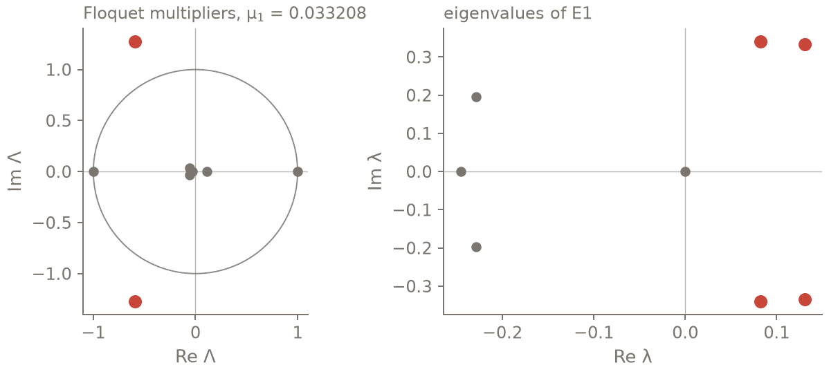
Stability of the solutions. Left: the multipliers of the orbit; the red pair outside the unit circle is the unstable direction, μ₁ = log|Λ|/T. Right: the leading eigenvalues of E1.

Check against the references

Energies and leading eigenvalues of \(E_1\) and \(E_2\), the speed and energy of \(TW_1\), and the leading Floquet exponent of \(\overline{pp}_{10.25}\) agree with the published digits; every solution is reported with its Newton residual.

assert E1.residual < 1e-12 and abs(E1.energy - 0.2609) < 6e-5
assert E2.residual < 1e-12 and abs(E2.energy - 0.4382) < 6e-5
for lam in (0.1308 + 0.3341j, 0.0824 + 0.3402j):            # Table 5.1 (to 4 digits)
    assert np.min(np.abs(ev1 - lam)) < 6e-5 or np.min(np.abs(ev1 - np.conj(lam))) < 6e-5
assert TW1.residual < 1e-12 and abs(TW1.params["c"] - 0.73699) < 6e-6
assert abs(TW1.energy - 0.4649) < 6e-5
assert ppo.residual < 1e-10 and abs(mu1 - 0.033209) <= 1e-6 and abs(theta1 - 2.0079) <= 1e-4
print("OK: E1, E2, TW1 and ppo_10.25 agree with the published digits")

Output (as executed)

# t05_ks_orbits: PASS (exit 0) in 68.7 s | 2026-10-20 | script sha256 1481734c97ed43b4
equilibrium: space=antisymmetric subspace R u = u (cos components frozen at 0), mean frozen
  relative residual 1.385e-16 (7 Newton iterations), energy E = 0.260873, status provisional
  note: residual = ‖v(u)‖/‖u‖ with v = M⁻¹(F − L u), evaluated in the full space
  note: trivial-state threshold: ‖u‖ < 1e-08 × 1 ⇒ retracted
E1: energy 0.2609, residual 1.4e-16; leading eigenvalues [0.1308-0.3341j 0.1308+0.3341j 0.0824-0.3402j 0.0824+0.3402j]
E2: energy 0.4382, residual 7.1e-16
TW1: c = 0.73699, energy 0.4649, residual 2.5e-16
ppo: T = 10.252881, residual 9.5e-14; mu_1 = 0.033208, theta_1 = 2.0079
OK: E1, E2, TW1 and ppo_10.25 agree with the published digits

Going further

• Continuation of the equilibria in \(L\) and their bifurcation points (KSDomainContinuation, tests/continuation/test_ks_L.py).

• Is an instability of a symmetric solution symmetry-breaking? symmetry_breaking_check (3. Symmetries and symmetry subspaces).

• Kolmogorov flow in 2D: tests/ecs/test_kolmogorov.py.