1. A first eigenvalue problem: Orr–Sommerfeld
Goal. Compute the least stable mode of plane Poiseuille flow at \(Re = 10^4\), \(\alpha = 1\), and
the critical Reynolds number, with a residual for every number.
Expected. \(c = 0.23752649 + 0.00373967\,i\) and \(Re_c = 5772.22\), \(\alpha_c = 1.02056\)
(Orszag 1971, J. Fluid Mech. 50, 689). Time: under a minute on one CPU core.
Script: t01_orr_sommerfeld.py.
The equation
For a normal mode \(v(y)\,e^{i\alpha(x - ct)}\) of the wall-normal velocity, with \(U = 1 - y^2\) and \(\mathcal{L}_2 = D^2 - \alpha^2\),
The eigenvalue \(c\) appears linearly; Conatus reads the mass matrix off its coefficient.
Write the problem
import conatus as cn
from conatus.expert import critical, verify
line = cn.Box(y=cn.walls(-1, 1))               # wall-normal coordinate y in [-1, 1]
m = cn.Model(line, name="Orr-Sommerfeld", Re=1e4, alpha=1.0)
m.scalar("v")                                  # v(y) exp(i alpha (x - c t)), wall-normal velocity
m.given(U=lambda y: 1 - y**2)                  # plane Poiseuille base flow (depends on y)
m.eigenvalue("c", growth="imag")               # wave speed c: a mode grows with Im c
m.define("L2(f) = dy(dy(f)) - alpha**2*f")     # D^2 - alpha^2
m.equations("Orr_Sommerfeld: L2(L2(v))/(1j*alpha*Re) - U*L2(v) + dy(dy(U))*v + c*L2(v) = 0")
m.at("walls", "v = 0", "dy(v) = 0")            # rigid walls at y = -1 and y = 1
print(m.explain(full=True))                    # every automatic decision (taus, modes)
Things to notice:
No basis, no size, no tau:
cn.Box(y=cn.walls(-1, 1))names the geometry,m.given(U=lambda y: 1 - y**2)the base flow (its argument names say it depends on \(y\) only),m.eigenvalue("c", growth="imag")the eigenvalue and how a mode grows (Im \(c\) for a phase speed;growth="real"for \(e^{st}\)),m.definethe operator \(\mathcal{L}_2\). The resolution is chosen when solving (N=64).m.at("walls", "v = 0", "dy(v) = 0")gives four conditions; each tau is placed by a fixed rule (in the equation where \(v\) has its highest order, modes \(N-1, \dots, N-4\)) andm.explain(full=True)prints them (m.explain()is the short summary). The matrices are bit-identical to the hand-written IR version (expert/t01_orr_sommerfeld.py,add_bc), which the test suite checks.
Solve and reject spurious modes
res = m.eigenvalues(N=64, drift=96, drift_tol=1e-6)   # keep modes found again at N = 96
i = int(res.values.imag.argmax())                     # least stable surviving mode
print(res.explain(key="imag"))
print(f"c = {res.values[i]:.10f}   backward residual {res.residuals[i]:.1e}")
The tau method produces spurious eigenvalues with huge \(|c|\). Conatus never hides them behind a
threshold: drift=96 (i.e. drift_plan=) solves the same problem at a finer resolution and keeps only modes that
reappear within drift_tol. res.explain() says how many modes were removed and why, and every
kept mode carries its backward residual \(\|(L + cM)x\|\) and its drift.
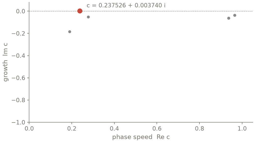
The modes kept by the drift test of the page (found again at N = 96), in the plane of phase speed and growth. Only one lies above the dashed line: the Tollmien-Schlichting wave, unstable at Re = 10⁴.
Plot the eigenfunction
mode = res.mode(i)                             # the eigenfunction on the grid, taus left out
print(mode.explain())                          # unknowns, grid, declared normalisation
y, v = mode.coordinate("y"), mode["v"]         # Chebyshev points, complex v(y)
res.mode(i) unpacks the eigenvector into the named unknowns on the physical grid: the tau
variables are left out, mode["v"] holds the complex values \(v(y_j)\) at the Chebyshev points
mode.coordinate("y"), and mode.coeffs("v") the Chebyshev coefficients. An eigenvector is only
defined up to a complex factor, so the normalisation is declared and printed by mode.explain():
the first unknown has \(\max|v| = 1\), real and positive where \(|v|\) is largest (here the centre of
the channel). The physical perturbation is \(\operatorname{Re}[v(y)\,e^{i\alpha(x - ct)}]\).
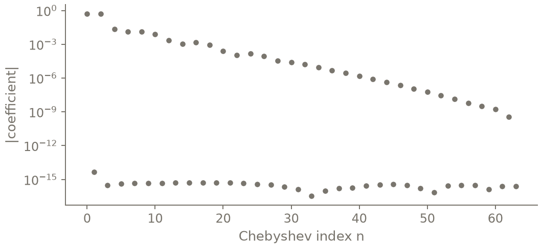
The Chebyshev coefficients of the mode (mode.coeffs(“v”)). The even ones fall to about 10⁻¹² by the last index, the level of the odd ones, which v, even in y, does not need: 64 modes resolve it.
Critical Reynolds number, sensitivity, verification
# L(Re, alpha) + c M(Re, alpha), exact in the parameters; the same pencil at N = 96 rejects the
# spurious tau modes (drift test, as for eigenvalues above); growth = Im c (the phase speed c)
P = m.parametric(N=64, over=("Re", "alpha"), drift=96, drift_tol=1e-6)
least = P.least_stable(Re=1e4, alpha=1.0)
crit = critical(P, "Re", bracket=(5000, 7000), over={"alpha": (0.98, 1.06)}, xtol=1e-9)
print(crit.explain())                          # growth convention, drift counts, verification
print(f"Re_c = {crit.value:.4f}   alpha_c = {crit.over['alpha']:.6f}")
print(f"dc/dRe = {P.sensitivity(least, 'Re'):.3e}")
print(verify(P, crit.mode, crit).explain())  # residuals, spectral tail, Taylor tests
ParametricEVP builds \(L(Re, \alpha)\) and \(M(Re, \alpha)\) once, as exact Laurent polynomials in the
parameters. drift=96 builds the same pencil at \(N = 96\): as for eigenvalues(drift=), only the
modes found again there within drift_tol are candidates, so the spurious tau modes never compete
with the physical ones (no hand-written bound on \(|c|\)). The growth of a mode is
\(\operatorname{Im} c\) because \(c\) is a phase speed: critical and least_stable read this off the
declared eigenvalue (m.eigenvalue("c", growth="imag")) and print it in crit.explain(). critical follows the least
stable mode by bordered Newton to \(\operatorname{Im} c = 0\) and minimises over \(\alpha\); a call that
leaves out a parameter of the pencil uses the value declared in the model (logged).
P.sensitivity gives \(\partial c / \partial Re\) from the left and right eigenvectors (no finite
differences). verify then reports residuals, the spectral tail of the eigenvector (is \(N = 64\)
enough?) and Taylor tests of the exact derivatives. A bracket in which the growth does not change
sign is refused with the growth at both ends and a suggested bracket.
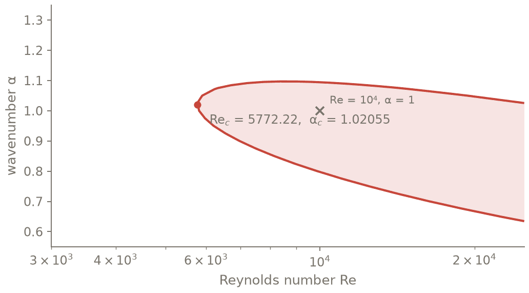
Im c of the least stable mode on a grid of (Re, α), from the parametric pencil of the page. Inside the red line the flow is unstable; its nose is the critical point the script finds.
Check against the reference
Check. \(c = 0.2375264888 + 0.0037396706\,i\) with backward residual \(4\times10^{-16}\), equal to Orszag’s \(0.23752649 + 0.00373967\,i\) to all eight published digits; \(Re_c = 5772.2218\) (Orszag: 5772.22), \(\alpha_c = 1.020547\) (Orszag: 1.02056).
C_ORSZAG = 0.23752649 + 0.00373967j          # Orszag (1971), Re = 1e4, alpha = 1
RE_C, ALPHA_C = 5772.22, 1.02056             # Orszag (1971); accurate value 1.020547
assert abs(res.values[i] - C_ORSZAG) < 1e-8, res.values[i]
assert res.residuals[i] < 1e-12
assert abs(abs(v).max() - 1) < 1e-14 and abs(v[0]) < 1e-3 and abs(v[-1]) < 1e-3   # normalised, v = 0 at the walls
assert abs(crit.value - RE_C) < 0.01 and abs(crit.over["alpha"] - ALPHA_C) < 2e-5
print("OK: c and Re_c agree with Orszag (1971) to the published digits; alpha_c within 2e-5")
Output (as executed)
# t01_orr_sommerfeld: PASS (exit 0) in 29.6 s | 2026-10-20 | script sha256 60324eaa146e273f
Model 'Orr-Sommerfeld'
Geometry: Box(y=walls(-1, 1)) (Cartesian box)
  bases (fixed per geometry, sizes given at discretization):
    y: walls at -1, 1 -> Chebyshev T(N_y)
  named boundaries: bottom = y left; top = y right; y=-1 = y left; y=1 = y right; walls = y left, y right
Unknowns: v (scalar)
Parameters: Re = 10000, alpha = 1 (change: m.<name> = value; for one call: simulate(..., name=value))
Given fields: U
Eigenvalue: c (complex); growth = Im c, declared with the eigenvalue c
Operator: L2(f) = dy(dy(f)) - alpha**2*f
Equations as written:
  [0] Orr_Sommerfeld: L2(L2(v))/(1j*alpha*Re) - U*L2(v) + dy(dy(U))*v + c*L2(v) = 0
Conditions as written:
  at walls: v = 0
  at walls: dy(v) = 0
Problem kind: EVP (eigenvalue c declared)
Term placement:
  [0] Orr_Sommerfeld
      operator  (1j*alpha*Re)**-1*(dy(dy(-alpha**2*v + dy(dy(v)))) - (-alpha**2*v + dy(dy(v)))*alpha**2)   (linear, constant coefficients)
      operator  c*(-alpha**2*v + dy(dy(v)))   (linear, constant coefficients)
      operator  dy(dy(U))*v   (linear, non-constant coefficient U)
      operator  -(-alpha**2*v + dy(dy(v)))*U   (linear, non-constant coefficient U)
Boundary conditions -> tau terms (automatic, deterministic):
  v = 0 at walls (left: y=-1): tau_v1 lifted into mode N_y-1 of [0] Orr_Sommerfeld -- v has its highest y-order (4) there; Chebyshev lift into the last modes
  v = 0 at walls (right: y=1): tau_v2 lifted into mode N_y-2 of [0] Orr_Sommerfeld -- v has its highest y-order (4) there; Chebyshev lift into the last modes
  dy(v) = 0 at walls (left: y=-1): tau_v3 lifted into mode N_y-3 of [0] Orr_Sommerfeld -- v has its highest y-order (4) there; Chebyshev lift into the last modes
  dy(v) = 0 at walls (right: y=1): tau_v4 lifted into mode N_y-4 of [0] Orr_Sommerfeld -- v has its highest y-order (4) there; Chebyshev lift into the last modes
Dealiasing: y: 3/2 (declared default 3/2 of the native layer: max(3/2, (p+1)/2) for the highest polynomial degree p = 2 of the equations in the unknowns and the given fields; on Fourier and polynomial bases a product of p fields, each truncated at the N modes of the resolution, is then computed without aliasing (a given field that is not resolved at N modes is truncated first: check its spectral tail); override with dealias=)
Bases: Chebyshev(y, size=8, bounds=(-1.0, 1.0), dealias=3/2)
Resolution: not chosen yet (simulate/eigenvalues/discretize(N=...))
EVP result [single group (no Fourier direction)] (dense QZ (scipy.linalg.eig)): 7 finite modes kept by the filters below, 8 infinite (M singular on tau/boundary rows)
  spectral-tail test (default, spurious='tail'): 0 of 7 modes flagged as spurious tau or unresolved modes (relative energy in the last 0.1 of the wall-normal coefficients above SPURIOUS_TAIL_TOL = 0.001); they are kept and ranked last by order()
  kept 7 of 60 modes: resolution drift <= 1e-06 against 92 modes at the finer resolution; 53 unresolved or spurious (tau) modes removed
  growth: growth = Im c, declared with the eigenvalue c
  modes sorted by decreasing imag part:
  c =  2.375264888190e-01+3.739670622253e-03j  residual 1.4e-16, drift 6.9e-12
  c =  9.646309154726e-01-3.516727756364e-02j  residual 1.1e-16, drift 7.3e-11
  c =  9.646425099829e-01-3.518658363628e-02j  residual 2.4e-16, drift 1.7e-10
  c =  2.772043438891e-01-5.089872753274e-02j  residual 1.9e-16, drift 1.0e-09
  c =  9.363165149228e-01-6.320147641683e-02j  residual 1.1e-16, drift 3.0e-08
  c =  9.363517179150e-01-6.325156402158e-02j  residual 1.8e-16, drift 6.8e-08
  (2 more log line(s): pencil and infinite-eigenvalue checks, solver settings: explain(full=True))
c = 0.2375264888+0.0037396706j   backward residual 1.4e-16
EVPMode 0 [single group (no Fourier direction)]: eigenvalue 0.237526488819+0.00373967062225j, residual 1.4e-16
  unknowns: v (complex grid values on the non-dealiased grid, y: 64; tau variables left out)
  normalisation: max |q| = 1 for the first non-zero unknown (declaration order), real and positive at its largest grid value; the other unknowns scaled by the same complex factor (here: v, max |v| = 1 at its largest grid value)
CriticalPoint Re_c = 5772.221816 at alpha=1.020547442 (11 neutral-curve evaluations)
  start: Re = 6000 (bracket midpoint (default))
  tolerance: |dRe| <= 1e-09 |Re| + 2e-09
  growth = Im c, declared with the eigenvalue c
  bracket ends (least stable admissible mode, full QZ): growth -1.513e-03 at Re = 5000, 1.578e-03 at Re = 7000: a sign change, so a neutral point lies inside
  spectral-tail test passed 35 of 60 (SPURIOUS_TAIL_TOL = 0.001); the spectral-tail test set aside 2 mode(s) of larger growth than every mode it kept (largest: sigma = 0.01709588437+2424.532429j, growth 2.425e+03, tail 1.0e+00): spurious tau or unresolved modes; raise N, or spurious='none' to select them; drift test kept 13 of 60 (resolution drift <= 1e-06 against the finer pencil [single group (no Fourier direction)] size (100, 100)) finite modes (8 infinite)
  at the critical point: spectral-tail test passed 35 of 60 (SPURIOUS_TAIL_TOL = 0.001); the spectral-tail test set aside 2 mode(s) of larger growth than every mode it kept (largest: sigma = 0.01678228628+2495.520313j, growth 2.496e+03, tail 1.0e+00): spurious tau or unresolved modes; raise N, or spurious='none' to select them; drift test kept 14 of 60 (resolution drift <= 1e-06 against the finer pencil [single group (no Fourier direction)] size (100, 100)) finite modes (8 infinite)
  ParametricEVP [single group (no Fourier direction)] size (68, 68): Re: exponents -1..0 (nominal 10000.0), alpha: exponents -1..3 (nominal 1.0); 5 coefficient matrices from 10 plans at roots of unity (5 identically zero dropped); reconstruction error at an independent real point 1.5e-16 (refused above 1e-10); pencil L + sM: structural rank 68/68, regular at a generic s (equilibrated sigma_min/sigma_max = 1.1e-07); mode tracking: bordered Newton, declared defaults TRACK_TOL = 1e-13, TRACK_MAX_ITERATIONS = 30
  verification: full QZ at the critical point, tracked mode is the least stable admissible one (max growth -1.7e-15), residual 5.2e-20
  TrackedMode sigma = 2.640002595802e-01+8.153621244480e-18j at {'alpha': np.float64(1.0205474415859814), 'Re': np.float64(5772.221816217911)}: residual 5.2e-20 after 1 bordered-Newton iterations; left vector available (sensitivities)
Re_c = 5772.2218   alpha_c = 1.020547
dc/dRe = -4.213e-06+3.428e-07j
Verification report: 9 checks, 0 to investigate by hand
  [PASS] pencil reconstruction: 1.54e-16 (threshold 1e-10) — parametric L(p), M(p) vs a directly assembled plan
  [PASS] pencil regular: 0.00e+00 (threshold 5e-01) — pencil L + sM: structural rank 68/68, regular at a generic s (equilibrated sigma_min/sigma_max = 1.1e-07)
  [PASS] right residual: 5.16e-20 (threshold 1e-12) — ||(L + sigma M) x|| backward error
  [PASS] left residual: 1.36e-20 (threshold 1e-12) — ||y^H (L + sigma M)|| backward error
  [PASS] spectral tail: 1.72e-10 (threshold 1e-08) — last 4 Chebyshev coefficients / max (mode resolved in N)
  [PASS] d sigma/d Re Taylor test: 4.44e-09 (threshold 1e-05) — exact sensitivity vs central difference of tracked sigma
  [PASS] d sigma/d alpha Taylor test: 7.60e-09 (threshold 1e-05) — exact sensitivity vs central difference of tracked sigma
  [PASS] critical point mode: 0.00e+00 (threshold 5e-01) — full QZ at the critical point confirms the tracked mode is the least stable
  [PASS] critical growth: 8.15e-18 (threshold 1e-10) — growth of the tracked mode at the neutral value
OK: c and Re_c agree with Orszag (1971) to the published digits; alpha_c within 2e-5
Going further
Same problem with shift-invert (
eigenvalues(plan, method="shift-invert", target=0.24, n_modes=4)).Left eigenvectors and the physical adjoint: IR and operators.
Symmetric subspaces of the same problem (half the cost): 3. Symmetries and symmetry subspaces.