16. Lagrangian tracers and a numerical dye
Tracers show where the fluid goes; a dye shows how it mixes. Both are only as good as the velocity they are given and the way they are advanced, so both are declared: the velocity at a tracer is the spectral series itself, the time integration has a stated order that the tutorial measures, and the dye is one more unknown of the model whose mass is written to its file.
Goal. Follow tracers in decaying Taylor–Green vortices and measure the order in time against a
path integrated to \(10^{-13}\); then shear a dye blob in plane Couette flow with tracers on the walls,
and read both files back with xarray.
Expected. Error divided by \(2^3\) when \(dt\) is halved (unsteady flow; \(2^4\) in a steady one);
Couette tracers \(x(t) = x_0 + y_0 t\) to rounding; dye mass conserved. Time: under a minute.
Script: t16_particles_dye.py · Tests behind it:
tests/model/test_particles_dye.py, tests/model/test_particles_gpu.py.
Tracers in an exact Navier–Stokes solution
nu, T = 0.5, 2.0


def taylor_green(dt):
    box = cn.Box(x=cn.periodic(2 * np.pi), y=cn.periodic(2 * np.pi))
    m = cn.Model(box, name="decaying Taylor-Green", nu=nu)
    m.velocity("u"), m.pressure("p")
    m.equations("dt(u) + grad(p) - nu*lap(u) = -u@grad(u)", "div(u) = 0")
    sim = m.simulate(N=(16, 16), scheme="RK443", dt=dt)
    sim.initial(u=lambda x, y: (np.sin(x) * np.cos(y), -np.cos(x) * np.sin(y)))
    return sim


X0 = np.random.default_rng(0).uniform(0, 2 * np.pi, (32, 2))
s = (1 - np.exp(-2 * nu * T)) / (2 * nu)


P = len(X0)


def path(_t, Z):
    x, y = Z[:P], Z[P:]
    return np.concatenate([np.sin(x) * np.cos(y), -np.cos(x) * np.sin(y)])


ref = solve_ivp(path, (0, s), np.concatenate([X0[:, 0], X0[:, 1]]), method="DOP853",
                rtol=1e-13, atol=1e-13).y[:, -1]
ref = np.stack([ref[:len(X0)], ref[len(X0):]], axis=1)
errors = []
for dt in (0.1, 0.05, 0.025):
    sim = taylor_green(dt)
    tracers = sim.particles(X0)
    sim.run(until=T)
    errors.append(np.abs(tracers.positions(unwrapped=True) - ref).max())
    print(f"dt = {dt:<6}: largest tracer error {errors[-1]:.2e}")
orders = np.log2(np.array(errors[:-1]) / np.array(errors[1:]))
print("observed orders:", np.round(orders, 2))
print(tracers.explain())
sim.particles(X0) registers the tracers with the simulation: each run step advances them by one
RK4 step. RK4 needs the velocity at the start, the middle and the end of the step; the ends are the
flow states themselves, the middle is interpolated in time through the last four flow states
(cubic, accurate to \(O(dt^4)\)). The order is 3 here because the flow states are only third-order
accurate in time (RK443), and because the first step of a run has only two states to interpolate
between; in a steady flow neither matters and the order is that of RK4, 4. With the velocity frozen
over a step it would be 1.
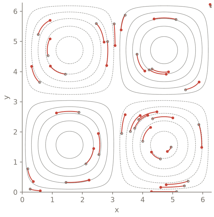
The 32 tracers of the page in the decaying Taylor-Green vortices, t = 0 to 2 (dt = 0.025): each moves along a streamline of ψ = sin x sin y (grey) and slows down as the flow decays.
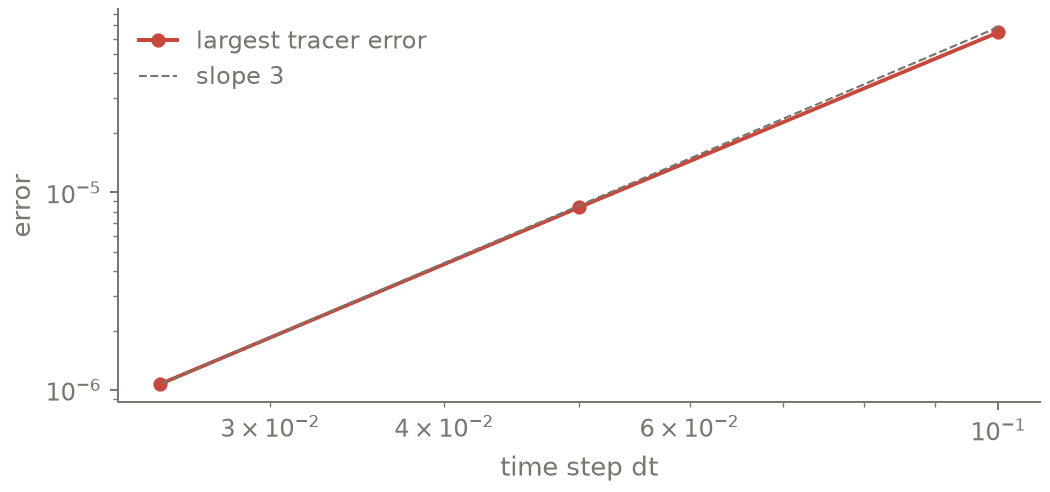
The tracer error against the reference path integrated to 10⁻¹³: third order in time, as stated for an unsteady flow.
A dye in plane Couette flow
box = cn.Box(x=cn.periodic(4.0), y=cn.walls(-1, 1))
m = cn.Model(box, name="plane Couette with dye", nu=0.1)
m.velocity("u"), m.pressure("p")
m.equations("dt(u) + grad(p) - nu*lap(u) = -u@grad(u)", "div(u) = 0")
m.at("bottom", u=(-1, 0))
m.at("top", u=(1, 0))
m.dye("c", velocity="u", kappa=0.01)      # dt(c) - 0.01*lap(c) = -div(c*u), dy(c) = 0 at walls
print(m.explain())
sim = m.simulate(N=(32, 32), scheme="RK443", dt=0.01)
sim.initial(u=lambda x, y: (y, 0 * x), c=lambda x, y: np.exp(-((x - 2) ** 2 + y ** 2) / 0.3))
out = Path(tempfile.mkdtemp())
starts = np.array([[0.0, -1.0], [1.0, -0.5], [2.0, 0.0], [3.0, 0.5], [0.5, 1.0]])
tracers = sim.particles(starts, path=out / "tracers.h5", every=50)
dye = sim.dye("c", out / "dye.h5", every=50)
sim.run(until=3.0)
print(dye.explain())
data = cn.io.read(out / "tracers.h5").to_xarray()
print(data["position_unwrapped"].isel(t=-1).values)
mass = cn.io.read(out / "dye.h5").tasks["mass"]
drift = np.abs(mass - mass[0]).max() / mass[0]
print(f"dye mass {mass[0]:.12f}, largest relative drift {drift:.1e}")
m.dye writes the dye’s equation in conservative form and its no-flux wall condition (both shown by
m.explain()); the dye is then advanced with the flow, by the same scheme. sim.dye writes it with
its mass, variance, extrema and spectral tail; sim.particles(..., path=, every=) writes positions
(wrapped and unwrapped), velocities and wall clips, with the dimensions t, particle,
component.
Check
assert np.all(orders > 2.6), orders                   # third order in an unsteady flow
exact = starts + np.column_stack([3.0 * starts[:, 1], 0 * starts[:, 1]])
assert np.abs(tracers.positions(unwrapped=True) - exact).max() < 1e-12
assert drift < 1e-8
print("checks passed: order 3 in time, Couette tracers exact, dye mass conserved")
Output (as executed)
# t16_particles_dye: PASS (exit 0) in 47.1 s | 2026-10-20 | script sha256 5421cf06aaa42843
dt = 0.1   : largest tracer error 6.46e-05
dt = 0.05  : largest tracer error 8.40e-06
dt = 0.025 : largest tracer error 1.07e-06
observed orders: [2.94 2.97]
Particles: 32 passive tracer(s) advected by u, backend cpu, 80 step(s) taken; no file (particles.positions())
  velocity at a particle: exact evaluation of the spectral series (x: cos/sin series (16 modes), y: cos/sin series (16 modes))
  time integration: classical RK4 per flow step; the midpoint velocity is the cubic interpolant in time of the last four flow states (2 and 3 states on the first two steps of a run): order 4 in a steady flow, 3 in an unsteady flow (the time error of the flow states themselves, third order for RK443, and the linear midpoint of the first step of a run)
  periodic axes: positions unwrapped (written also wrapped into [a, a + L))
  walls: at_walls='refuse' (a step ending outside the walls raises); stage positions are not clipped (the series continues there)
  not in the simulation's checkpoints: after a restart, declare the particles again (e.g. from the last row of the file)
Model 'plane Couette with dye': Box(x=periodic((0, 4)), y=walls(-1, 1)) (Cartesian box)
Unknowns: u (velocity), p (pressure), c (dye); parameters: nu = 0.1
Equations as written:
  eq0: dt(u) + grad(p) - nu*lap(u) = -u@grad(u)
  eq1: div(u) = 0
  dye_c: dt(c) - 0.01*lap(c) = -div(c*u)
Problem: IVP (a time derivative dt() appears)
Time stepping: 6 linear term(s) implicit; nonlinear terms explicit (eq0, dye_c)
Boundary conditions: bottom: u = (-1, 0); top: u = (1, 0); walls (left: y=-1): dy(c) = 0; walls (right: y=1): dy(c) = 0 (tau method, placed automatically)
Gauge: the mean of p is fixed (integ(p) = 0)
Dealiasing: x: 3/2, y: 3/2 (declared default for products of degree 2)
Resolution: not chosen yet (simulate/eigenvalues/discretize(N=...))
(every decision, tau by tau and term by term: m.explain(full=True))
Dye file <path>/tmp62lfbd_4/dye.h5 (HDF5, conatus.analysis/1): every 50 steps (= 0.5 time units), 7 write(s) so far
  dye c (m.dye): dt(c) - 0.01*lap(c) = -div(c*u); no flux: dy(c) = 0 at the walls; advected by u, same scheme and dt as the flow
  c: grid values of c
  mass: integ(c) (integral of the spectral series)
  variance: integ(c*c) - integ(c)^2 / V, V = 8
  minimum: min of the grid values of c
  maximum: max of the grid values of c
  tail: largest |coefficient| among the last two modes of each axis, relative to the largest
  the state at the start (iteration 0, t = 0) written as a row (initial=True, the default of sim.output)
  scales: sim_time, iteration, write_number, x, y; every array labelled with its dimensions (HDF5 dimension scales)
  XDMF sidecar (ParaView): <path>/tmp62lfbd_4/dye.xmf
[[-3.  -1. ]
 [-0.5 -0.5]
 [ 2.   0. ]
 [ 4.5  0.5]
 [ 3.5  1. ]]
dye mass 0.933219300417, largest relative drift 1.1e-11
checks passed: order 3 in time, Couette tracers exact, dye mass conserved
Going further
Guide: Particles and dye of a simulation (walls, files, GPU, what is not covered).
Streaklines, timelines, inertial particles and FTLE from snapshots: Diagnostics and visualization.