10. Bifurcations: branch switching, cycles, codimension 2, normal forms¶
Goal. Build the bifurcation diagram of the Lorenz system (pitchfork with a declared symmetry,
Hopf point, its first Lyapunov coefficient, the cycles born there), follow fold and Hopf curves of
the Bogdanov–Takens normal form in two parameters, and derive the Landau and Ginzburg–Landau
coefficients of Swift–Hohenberg rolls.
Expected. Lorenz (1963): pitchfork at \(r = 1\) with \(x^2 = b(r-1)\) on \(C^\pm\); Hopf at
\(r_H = \sigma(\sigma+b+3)/(\sigma-b-1) = 470/19\) with \(\omega^2 = b(\sigma + r_H)\), subcritical
(Marsden & McCracken 1976). Bogdanov–Takens (Kuznetsov 2004, §8.4): fold curve \(\beta_1 = \beta_2^2/4\),
Hopf curve \(\beta_1 = 0\), both ending at \((0,0)\). Swift–Hohenberg (Cross & Hohenberg 1993):
\(A^2 = 4r/3\), \(\tau_0 = 1\), \(\xi_0^2 = 4\), \(g_0 = 3\). Time: under a minute on one CPU core.
Script: t10_bifurcations.py · Tests behind it:
tests/bifurcation/test_bifurcation_core.py, tests/bifurcation/test_amplitude.py.
Write the system¶
lorenz = ode_problem(["x", "y", "z"], {"sigma": 10.0, "r": 0.5, "b": 8 / 3},
                     lambda X, P: [P["sigma"] * (X["y"] - X["x"]),
                                   P["r"] * X["x"] - X["y"] - X["x"] * X["z"],
                                   X["x"] * X["y"] - P["b"] * X["z"]], name="Lorenz")
L = ir_system(lorenz, ["r"])          # G(x; r), exact J, dG/dr, and the multilinear forms B, C
print(L.explain())
ode_problemwrites an ODE from its right-hand side, given as a Python function of the state and the parameters. A PDE written as a native model works the same way (Swift–Hohenberg below).ir_systemdiscretizes once and exposes \(M\dot x = G(x;p)\). The Jacobian and the multilinear forms \(B = F''\), \(C = F'''\) are exact symbolic Fréchet derivatives of the equations: no finite differences in \(x\). \(\partial G/\partial r\) is exact too: the equations say that \(r\) enters linearly, andexplain()says so.
Equilibria and branch switching with a declared symmetry¶
cfg = ContinuationSettings(ds=0.1, ds_min=1e-9, ds_max=2.0, adapt=1.3, fast_iterations=4,
                           tolerance=1e-11, max_newton=12, max_points=60, dp_fd=None)
origin = continue_equilibria(L, np.zeros(3), "r", cfg, marginal_tol=1e-9, bounds=(0, 3))
(bp,) = origin.events_of("branch point")
S = np.diag([-1.0, -1.0, 1.0])        # (x, y, z) -> (-x, -y, z): a symmetry of Lorenz, declared
cplus = branch_switch(origin, bp, cfg, step=0.05, symmetry=S, bounds=(0, 30))
print(cplus.explain())
(hopf,) = cplus.events_of("hopf")
continue_equilibria evaluates three test functions at every point (fold: the parameter component of
the tangent; branch point: the determinant of the bordered Jacobian; Hopf: a product over eigenvalue
pairs) and locates each sign change by a secant, reporting the residual there. branch_switch
solves the algebraic branching equation with the exact second derivatives; the declared
\(S = \mathrm{diag}(-1,-1,1)\) classifies the point as a symmetry-breaking pitchfork: the kernel is
\(S\)-odd, and the two half-branches \(C^\pm\) are images of each other. Nothing is guessed from a plot.
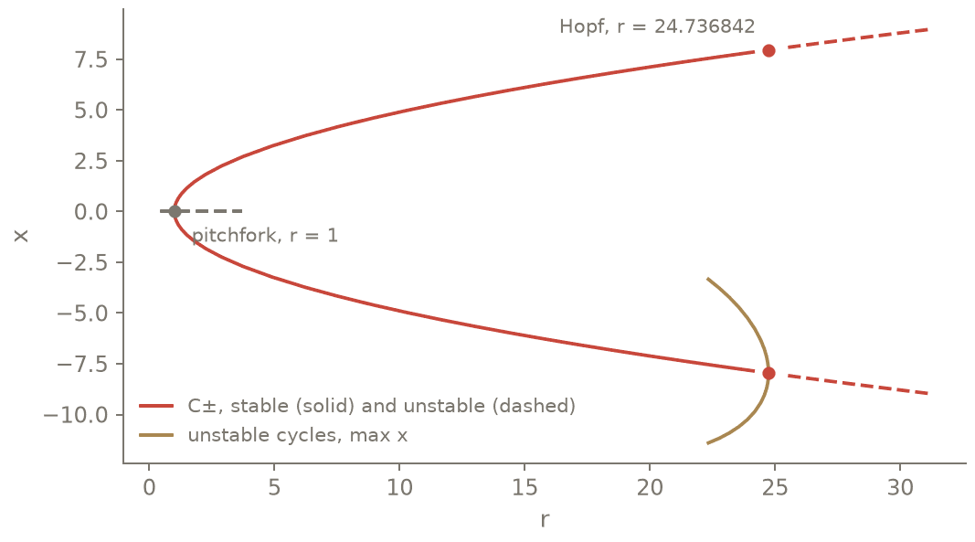
The equilibria of the Lorenz system and their stability, as continued by the page: the origin, the pitchfork at r = 1, the branches C± and their subcritical Hopf points, and the cycles born there.¶
Normal forms¶
pf = normal_form(L, bp.point.z[:-1], kind="zero", par={"r": bp.point.z[-1]}, parameter="r", symmetry=S)
hf = normal_form(L, hopf.point.z[:-1], kind="hopf", par={"r": hopf.point.z[-1]}, parameter="r")
print(pf.explain())
print(hf.explain())
The centre-manifold projection (Kuznetsov) gives the pitchfork cubic coefficient and, at the Hopf point, \(c_1\) and the first Lyapunov coefficient \(\ell_1 = \mathrm{Re}\,c_1/\omega\): positive here, so the Hopf bifurcation of Lorenz is subcritical. Every quantity is reported with its checks (residuals of the eigenvectors and of the bordered solves); the normalization \(\|q\| = 1\) is declared.
Cycles from the Hopf point¶
cfo = ContinuationSettings(ds=0.2, ds_min=1e-9, ds_max=1.0, adapt=1.3, fast_iterations=4,
                           tolerance=1e-9, max_newton=12, max_points=12, dp_fd=None)
cycles = branch_switch(cplus, hopf, cfo, amplitude=0.2, mesh=CollocationMesh.uniform(40, 4),
                       tests=("lpc",))
print(cycles.explain())
The first cycle is predicted by the normal form (amplitude declared, \(\Delta r = -\mathrm{Re}\,c_1|z|^2/\alpha'\)), corrected by orthogonal collocation (AUTO’s method) and continued. Subcritical: the cycles exist for \(r < r_H\). Followed further, their period diverges at the homoclinic explosion \(r \approx 13.926\).
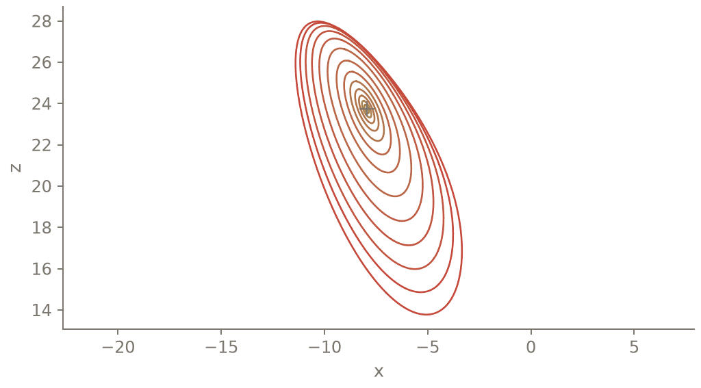
The periodic orbits of the cycle branch (orthogonal collocation, 40 intervals of degree 4) for r from 24.735 down to 22.335: born at the Hopf point around the equilibrium of the continued branch (cross), they grow as r decreases.¶
Two parameters: fold and Hopf curves¶
bt = ir_system(ode_problem(["x", "y"], {"b1": -0.5, "b2": -1.0},
                           lambda X, P: [X["y"], P["b1"] + P["b2"] * X["x"] + X["x"] * X["x"]
                                         - X["x"] * X["y"]], name="Bogdanov-Takens"), ["b1", "b2"])
cfg2 = ContinuationSettings(ds=0.05, ds_min=1e-9, ds_max=0.3, adapt=1.3, fast_iterations=3,
                            tolerance=1e-11, max_newton=12, max_points=40, dp_fd=None)
eq = continue_equilibria(bt, np.array([(1 - np.sqrt(3)) / 2, 0.0]), "b1", cfg2, marginal_tol=1e-9,
                         bounds=(-2, 2))
fold_pt, hopf_pt = eq.events_of("fold")[0], eq.events_of("hopf")[0]
fold_curve = continue_codim2(bt, fold_pt.point.z[:-1], "fold", ("b1", "b2"), cfg2,
                             par={"b1": fold_pt.point.z[-1]}, bounds={"b2": (-1.5, 1.5)})
hopf_curve = continue_codim2(bt, hopf_pt.point.z[:-1], "hopf", ("b1", "b2"), cfg2,
                             par={"b1": hopf_pt.point.z[-1]}, bounds={"b2": (-1.5, 1.5)})
print(fold_curve.explain())
print(hopf_curve.explain())
Minimally augmented systems (Govaerts): one scalar condition \(g = 0\) from a bordered matrix (fold), two for Hopf (bordered \(J^2 + \kappa I\), \(\kappa = \omega^2\)). Along the curves, test functions detect cusp, Bogdanov–Takens, Bautin, fold–Hopf and Hopf–Hopf points; here both curves end at the BT point, and the vanishing determinant there is not reported as a fold–Hopf point (rejected with its reason).
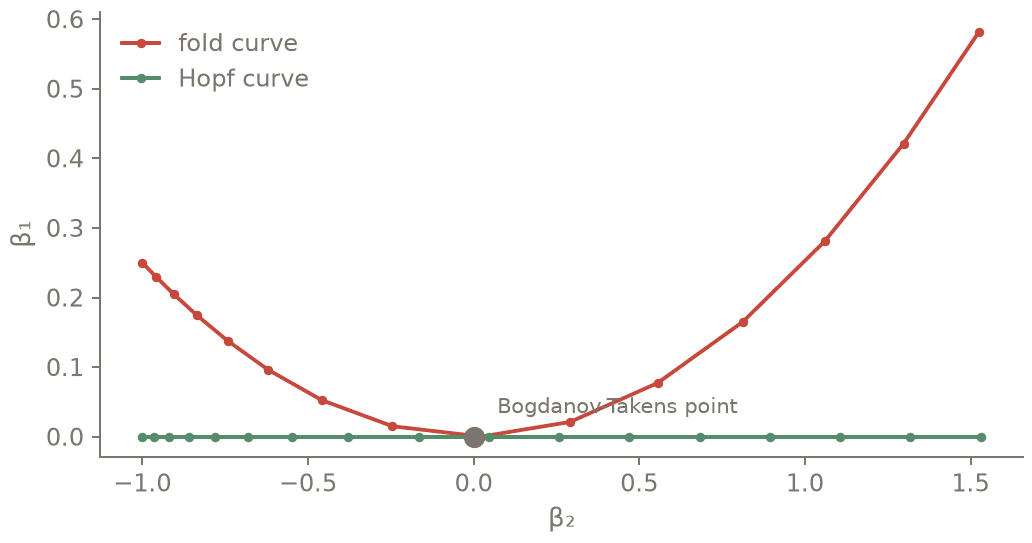
Codimension two: the fold and Hopf curves of the Bogdanov-Takens normal form, continued in (β₁, β₂). The fold curve follows β₁ = β₂²/4, the Hopf curve β₁ = 0; both end at the BT point.¶
Landau and Ginzburg–Landau equations of a PDE¶
def swift_hohenberg(k, N=16):
    """Swift-Hohenberg on one wavelength 2 pi / k, as a native model; r is the free parameter."""
    m = cn.Model(cn.Box(x=cn.periodic(2 * np.pi / k)), name="Swift-Hohenberg", r=0.0)
    m.scalar("u")                                          # the unknown
    m.define("S(f) = f + dx(dx(f))")                       # (1 + d_xx), a named operator
    m.equations("dt(u) - r*u + S(S(u)) = -u*u*u")
    c = m.compile(N, dealias=2)                            # u^3: dealias 2, declared
    # The even subspace u(-x) = u(x) (pins the phase of the rolls) is declared on the compiled
    # problem: the native layer has no symmetry= option yet.
    even = IVP(c.problem.variables, name=c.problem.name,
               symmetry=SymmetrySubspace(Reflection(c.coordsys["x"], about=0), u=EVEN))
    for eq in c.problem.equations:
        even.add_equation(eq)
    s = ir_system(even, ["r"])
    return s, np.zeros(s.n)


sh, u0 = swift_hohenberg(1.0)
cos_coeff = cos_mode_observable(sh, "u")          # A = coefficient of cos x in u (linear functional)
landau = amplitude_equation(sh, u0, "r", kind="stationary", observable=cos_coeff)
gl = ginzburg_landau(swift_hohenberg, 1.0, "r", kind="stationary", observable=cos_coeff, h=1e-2)
print(landau.explain())
print(gl.explain())
Swift–Hohenberg is a native model: the operator \(1 + \partial_{xx}\) is named once with
m.define, the equation is written as on paper, and dealias=2 is written out although it is
the native default for a cubic nonlinearity ((p+1)/2 with p = 3): the published coefficients do not
depend on a default. The even subspace \(u(-x) = u(x)\) removes the translation mode; it is declared
on the compiled problem (expert layer), because the native layer has no symmetry= option yet.
amplitude_equation rewrites the pitchfork normal form for an observable amplitude (here the
\(\cos x\) coefficient), and ginzburg_landau adds the curvature of the growth rate \(\sigma(k)\)
(systems rebuilt at \(k_c \pm h\), \(\pm 2h\), fourth-order differences, step declared). The same call
on stress-free Rayleigh–Bénard rolls gives \(\mathrm{Nu} - 1 = 2\varepsilon\) (Malkus & Veronis 1958)
with spectral convergence in \(N_z\): examples/bifurcation/weakly_nonlinear.py.
Check against the closed forms¶
The pitchfork at \(r = 1\), the branch \(x^2 = b(r-1)\), the Hopf point \(r_H = 470/19\) with its frequency and a positive first Lyapunov coefficient, the fold and Hopf curves of the Bogdanov–Takens normal form, and the Swift–Hohenberg coefficients \(A^2/r = 4/3\), \(\xi_0^2 = 4\), \(g_0 = 3\) are all recovered to rounding.
sig, b = 10.0, 8 / 3
rH = sig * (sig + b + 3) / (sig - b - 1)                        # 470/19, Lorenz (1963)
assert abs(bp.point.z[-1] - 1) < 1e-12 and cplus.switch["classification"] == "pitchfork (symmetry-breaking)"
xs = np.array([p.z[0] for p in cplus.points])
assert np.abs(xs ** 2 - b * (cplus.column("r") - 1)).max() < 1e-9          # C+: x^2 = b (r - 1)
assert abs(hopf.point.z[-1] - rH) < 1e-9 and abs(hf.omega ** 2 - b * (sig + rH)) < 1e-9
assert hf.l1 > 0                                                          # subcritical
assert cycles.column("r").max() < rH                                      # cycles exist for r < r_H
assert np.abs(fold_curve.column("b1") - fold_curve.column("b2") ** 2 / 4).max() < 1e-10
assert np.abs(hopf_curve.column("b1")).max() < 1e-12
assert np.abs(hopf_curve.events_of("bt")[0].point.z[-2:]).max() < 1e-10
assert abs(landau.g3 + 0.75) < 1e-12 and abs(gl.xi0_sq - 4) < 1e-9 and abs(gl.g0 - 3) < 1e-12
print(f"CHECK r_H = {hopf.point.z[-1]:.12f} (470/19 = {rH:.12f}), l1 = {hf.l1:.6e} > 0; "
      f"SH: A^2/r = {landau.amplitude(1.0) ** 2:.12f} (4/3), xi0^2 = {gl.xi0_sq.real:.10f}, g0 = {gl.g0.real:.12f}")
Output (as executed)¶
# t10_bifurcations: PASS (exit 0) in 28.7 s | 2026-10-20 | script sha256 1aeaf6f6d8fb15f0
DynamicalSystem: M dx/dt = G(x; p), n = 3, origin: IR: Lorenz (0-D: one constant Fourier mode)
  parameters: r = 0.5
  mass matrix: identity
  origin: IR (discretized IVP; F by the spectral evaluator, derivatives symbolic)
  IVPSolver used as evaluator/matrix container only: no time step is taken
  pointwise=True: 0-D system, IR expressions compiled to vectorised numpy (same expressions as the spectral evaluator)
  dG/dr (RHS): exact Laurent reconstruction, exponents [0, 1]
equilibrium curve: 32 points, r in [1.00047, 31.1039]; stop: r = 31.1039 left (0, 30)
  branch switch at r = 1: pitchfork (symmetry-breaking); ABE c = (0.000e+00, -7.036e-01, 0.000e+00), known-branch alignment 1.000000000000, step 0.05 (direction +1); first corrected point residual 2.2e-19; S φ = −φ on an S-invariant branch: the other half-branch is the S-image
  equilibria of IR: Lorenz (0-D: one constant Fourier mode) in r
  stability: #Re λ > 1e-09 (generalized eigenvalues of (J, M), |λ| > 1e+10(1 + max|J|) removed as infinite)
  tests: fold, branch point, hopf; Hopf test over 3 eigenvalue(s)
  ds = 0.1 in [1e-09, 2], x1.3 (default) when the corrector takes <= 4 its, /2 on failure
  corrector: tolerance 1e-11, budget 12 (default) its; G_p: analytic G_p (dp_fd=None)
  max points 60
  events: secant budget event_max_iterations = 30 (default), fold_tol = 1e-12 (default) (|t_p|), crossing_tol = 1e-11 (default) (|Re λ| / max(1, |λ|)), hopf_imag_tol = 1e-08 (default) (|Im λ| / max(1, |λ|))
  corrector failures (step halved): 0; max residual on the curve 8.4e-12
  hopf at r = 24.7368421053 between points (26, 27), |test| = 5.3e-13, residual 2.8e-14: λ = -3.00e-13 ± 9.62453006371 i [located by |test hopf| <= crossing_tol = 1e-11, secant budget 30]
Normal form (pitchfork (supercritical)) at r = 1: da/dt = μ Δp a + a3 a³
  β = 0, μ = 0.9090909091, a2 = 0, a3 = -0.1704545455
  x ≈ x0 + a q + a²/2 h2, ‖q‖ = 1 (declared norm), pᵀM q = 1
  check max|G(x0)|: 0.0e+00
  check |λ_0|: 0.0e+00
  check ‖J q‖: 2.2e-16
  check ‖pᵀJ‖: 2.2e-16
  check residual h2: 0.0e+00
  check residual x_p: 0.0e+00
  declared symmetry: S q = −q
Hopf normal form at r = 24.7368421053: ω = 9.62453006371
  c1 = 0.002555495334 -0.02765775717 i, first Lyapunov coefficient l1 = Re c1 / ω = 0.0002655189726 (subcritical)
  normalization: ‖q‖ = 1 (declared norm), pᴴM q = 1 (Kuznetsov); Re c1 / ‖q‖² is invariant
  λ'(r) = 0.03022248268 +0.1814503065 i -> Landau: dz/dt = λ' Δr z + c1 z|z|²
  check max|G(x0)|: 2.8e-14
  check |Re λ|: 3.0e-13
  check ‖(J − iωM) q‖: 2.2e-13
  check ‖pᴴ(J − iωM)‖: 2.3e-13
  check |pᴴ M q − 1|: 6.4e-17
  check Re h11 imag part: 0.0e+00
periodic orbit curve: 13 points, r in [22.3351, 24.7352], T in [0.652887, 0.748573]; stop: max_points = 12 reached
  Hopf → cycles at r = 24.7368421053 (ω = 9.624530064, l1 = 0.000265519, subcritical); predictor: amplitude 0.2 (declared), Δr = -1.6370e-03, T = 0.65288682; corrected at fixed r: T = 0.65288682
  periodic orbits of IR: Lorenz (0-D: one constant Fourier mode) in r: orthogonal collocation, ntst = 40, ncol = 4 (Gauss points), integral phase condition
  mesh: uniform, fixed
  arclength norm: nodes weighted 1/npts (discrete L2 in τ), T and p weight 1
  Floquet multipliers from the collocation monodromy (condensation); |μ_triv − 1| stored on every point; multipliers below 1e-08 x max(1, |μ|max) are unresolved (count stored) and left out of the tests
  stability: 'unstable' counts nontrivial |μ| > 1 + 1e-06; ||μ| − 1| <= 1e-06 is near-marginal (stored as 'marginal', listed below), not counted
  ds = 0.2 in [1e-09, 1], x1.3 (default) when the corrector takes <= 4 its, /2 on failure
  corrector: tolerance 1e-09, budget 12 (default) its; G_p: analytic G_p (dp_fd=None)
  max points 12
  events: secant budget event_max_iterations = 30 (default), fold_tol = 1e-12 (default) (|t_p|), crossing_tol = 1e-11 (default) (|Re λ| / max(1, |λ|)), hopf_imag_tol = 1e-08 (default) (|Im λ| / max(1, |λ|))
  corrector failures (step halved): 0; max residual on the curve 5.9e-10
  no event detected
fold (codim 2) curve: 15 points, b1 in [0.000137149, 0.58141], b2 in [-1, 1.52501]; stop: b2 = 1.52501 left (-1.5, 1.5)
  fold curve of IR: Bogdanov-Takens (0-D: one constant Fourier mode) in (b1, b2), minimally augmented system (Govaerts 2000); bordering vectors refreshed after every accepted point
  tests: cusp, bt, zh
  ds = 0.05 in [1e-09, 0.3], x1.3 (default) when the corrector takes <= 3 (default) its, /2 on failure
  corrector: tolerance 1e-11, budget 12 (default) its; G_p: analytic G_p (dp_fd=None)
  max points 40
  events: secant budget event_max_iterations = 30 (default), fold_tol = 1e-12 (default) (|t_p|), crossing_tol = 1e-11 (default) (|Re λ| / max(1, |λ|)), hopf_imag_tol = 1e-08 (default) (|Im λ| / max(1, |λ|))
  corrector failures (step halved): 0; max residual on the curve 1.4e-12
  bt at b1 = -6.7114253235e-16, b2 = 1.11699588465e-12 between points (7, 8), |test| = 5.6e-13, residual 6.7e-16 [located by |test bt| <= crossing_tol = 1e-11, secant budget 30]
hopf (codim 2) curve: 17 points, b1 in [1.90168e-14, 2.38022e-14], b2 in [-1, 1.53084], kappa in [-1.53084, 1]; stop: b2 = 1.53084 left (-1.5, 1.5)
  hopf curve of IR: Bogdanov-Takens (0-D: one constant Fourier mode) in (b1, b2), minimally augmented system (Govaerts 2000); bordering vectors refreshed after every accepted point
  tests: bt, gh, zh, hh
  Hopf conditions: entries (2, 3) of the 2x2 bordered G (row-major), chosen once at the start for the best-conditioned augmented Jacobian
  ds = 0.05 in [1e-09, 0.3], x1.3 (default) when the corrector takes <= 3 (default) its, /2 on failure
  corrector: tolerance 1e-11, budget 12 (default) its; G_p: analytic G_p (dp_fd=None)
  max points 40
  events: secant budget event_max_iterations = 30 (default), fold_tol = 1e-12 (default) (|t_p|), crossing_tol = 1e-11 (default) (|Re λ| / max(1, |λ|)), hopf_imag_tol = 1e-08 (default) (|Im λ| / max(1, |λ|))
  corrector failures (step halved): 0; max residual on the curve 1.4e-13
  bt at b1 = 1.90259931987e-14, b2 = -2.65065747129e-13, kappa = -5.55111512313e-17 between points (8, 9), |test| = 5.6e-17, residual 1.9e-14: κ = ω² = -5.55e-17 [located by |test bt| <= crossing_tol = 1e-11, secant budget 30]
  (rejected zh between (8, 9): det J = 0 with κ = ω² = -4.7e-16: the Bogdanov–Takens point)
Landau equation (stationary) at r_c = 0: dA/dt = μ Δr A + g3 A³
  μ = 1+0j, g3 = -0.75+0j (observable of q: 1+0j)
  A² = −Re μ Δp / Re g3 = 1.333333333 Δr
  from the pitchfork normal form: a3 / ℓ(q)², A = a ℓ(q)
Ginzburg–Landau at k_c = 1, r_c = 0:
  ∂t A = μ Δr A + v_g-term + D ∂X² A + g |A|² A, u = A e^(i k_c x) q + c.c.
  μ = 1+0j, D = −σ_kk/2 = 4-0j, v_g = -0, g = -3+0j
  Cross–Hohenberg form (ε = Δr): τ0 = 1, ξ0² = 4+0j, g0 = 3+0j
  σ_kk: 4th-order central differences, h = 0.01 (declared); |4th − 2nd order| = 1.0e-04
  g = 4 g3 (u = A e^{ikx} + c.c. = 2|A| cos kx)
CHECK r_H = 24.736842105253 (470/19 = 24.736842105263), l1 = 2.655190e-04 > 0; SH: A^2/r = 1.333333333333 (4/3), xi0^2 = 4.0000000000, g0 = 3.000000000000
Going further¶
Period doubling with branch switching onto the doubled orbit, Neimark–Sacker detection, branch points of cycles:
tests/bifurcation/test_bifurcation_core.py(constructed systems with exact multipliers).Continuation and bifurcations in the user guide: User guide.