4. Nonlinear boundary-value problems and continuation: Bratu

Goal. Solve the Bratu problem \(u'' + \lambda e^u = 0\) by Newton, see quadratic convergence reported, then follow the solution branch by pseudo-arclength continuation through its fold. Expected. The closed form \(u = 2\ln(\cosh a / \cosh a x)\), \(\lambda = 2a^2/\cosh^2 a\) (Bratu 1914; Gelfand 1963), with the fold at \(a \tanh a = 1\): \(\lambda_c = 0.87845767978129\ldots\) on \([-1, 1]\) (\(= 3.51383071912516/4\), the classical value on \([0, 1]\)). Time: a few seconds on one CPU core. Script: t04_bratu.py · Tests behind it: tests/nlbvp/test_nlbvp.py, tests/continuation/test_continuation.py::test_bratu_branch_through_the_fold.

The problem

\[ u'' + \lambda\, e^{u} = 0 \quad \text{on } [-1, 1], \qquad u(\pm 1) = 0 . \]

For \(\lambda < \lambda_c\) there are two solutions (lower and upper branch); they merge at the fold \(\lambda_c\) and none exists beyond. A Newton solver alone cannot pass the fold: the Jacobian is singular there. Pseudo-arclength continuation parametrises the branch by its arclength instead.

Write the problem

import numpy as np
from scipy.optimize import brentq

import conatus as cn
from conatus.expert import ContinuationSettings, NewtonSolver, NLBVPContinuation, grid

m = cn.Model(cn.Box(x=cn.walls(-1, 1)), name="Bratu", lam=0.3)
u = m.scalar("u")
m.equations("bratu: dx(dx(u)) + lam*exp(u) = 0")   # no dt(): a nonlinear boundary-value problem
m.at("walls", u=0)
print(m.explain())                               # kind, tau placement, dealiasing: all declared
pb = m.compile(64, dealias=1)                    # dealias declared: exp(u) is not alias-free anyway;
                                                 # 64 modes resolve exp(u) to 1e-12 up the upper branch

• The model has no dt(), and the equation is nonlinear in u: m.explain() reports a nonlinear boundary-value problem and keeps every term as written (there is no implicit/explicit split; Newton linearizes the whole residual). The two conditions u = 0 at the walls are placed by the same fixed rule as in a simulation, and listed.

• exp(u) has an exact Fréchet derivative (\(e^u\,\delta u\)), which is what Newton uses. It is not alias-free for any dealiasing factor, so the factor is declared (dealias=1) rather than left to the native default; resolution is then checked by convergence in \(N\), not assumed.

• m.compile(64, ...) returns the compiled problem: Newton and continuation act on pb.problem, and pb.fields["u"] names the unknown in the initial guess.

Newton

newton = NewtonSolver(pb.problem, tol=1e-13, damping=1.0, max_iterations=20, params={"lam": 0.3})
sol = newton.solve({pb.fields["u"]: lambda x: 0 * x})   # initial guess u = 0
print(sol.explain())                             # residual per iteration, observed orders

The tolerance tol is required: it decides the digits of the solution. The damping (default 1, full Newton steps) and the iteration budget (default 50) have declared defaults; the script gives both explicitly (1 and 20). All three are printed with the result. sol.explain() lists the residual of every iteration and the observed order of convergence \(q_k = \log(r_{k+1}/r_k)/\log(r_k/r_{k-1})\), about 2 here, the signature of an exact Jacobian. Non-convergence raises NewtonNotConverged with the history; it never returns the last iterate silently.

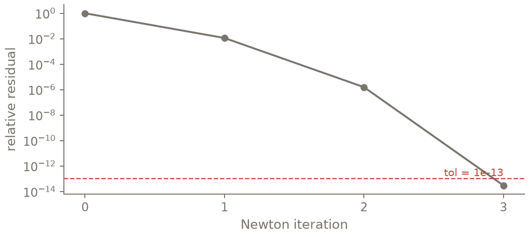
Newton from u = 0 at λ = 0.3, as printed by sol.explain(): the number of correct digits doubles at each step (quadratic convergence) down to the declared tolerance.

Continuation through the fold

settings = ContinuationSettings(ds=0.2, ds_min=1e-8, ds_max=0.6, adapt=1.5, fast_iterations=3,
                                tolerance=1e-12, max_newton=15, max_points=6, dp_fd=1e-6)
cont = NLBVPContinuation(newton, "lam", settings)
branch = cont.run(sol.coeffs, 0.3, +1, p_bounds=(0.3, 1.0))
print(branch.explain())
(fold,) = branch.folds()                          # located by bisection on the tangent
print(f"fold: lam_c = {fold.p:.14f}")

ContinuationSettings requires what sets the accuracy and the scale of the branch (step size and its bounds, corrector tolerance, number of points); the algorithm controls (adaptation factor, corrector budget, finite-difference step for \(\partial G/\partial\lambda\)) have declared defaults, marked “(default)” by explain(). The branch starts on the lower branch at \(\lambda = 0.3\), passes the fold and comes back down the upper branch for a few points (max_points). Up there \(u\) grows and \(e^u\) needs more modes: at 64 modes its Chebyshev tail stays below \(10^{-12}\) along the whole branch; at too few modes Conatus refuses the step (a non-constant coefficient whose Chebyshev tail exceeds ncc_tail_tol, \(10^{-8}\) by default, is never used or truncated silently: the error gives the resolution to use, or the ncc_cutoff= to declare). Folds are located (the \(\lambda\)-component of the tangent changes sign, refined to \(|t_\lambda| \approx 10^{-16}\)), not read off the nearest point; branch.explain() reports the residual at the located point and every step-size change.

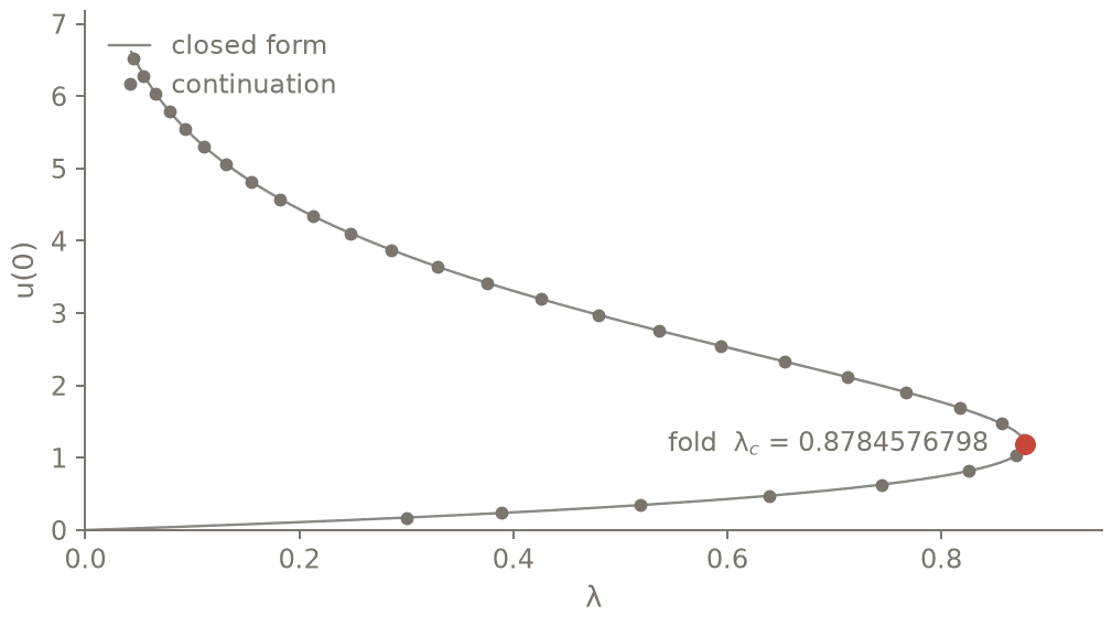
The branch followed by pseudo-arclength continuation (the page’s settings, run for more points), on the closed form u(0) = 2 ln cosh a. The fold is located by bisection on the tangent.

Check against the closed form

Newton converges quadratically to the closed-form lower-branch solution, and the located fold agrees with the root of \(a\tanh a = 1\) to rounding.

a_star = brentq(lambda a: a * np.tanh(a) - 1.0, 0.5, 2.0, xtol=1e-15)
LAM_C = 2 * a_star ** 2 / np.cosh(a_star) ** 2   # 0.87845767978129...
a03 = brentq(lambda a: 2 * a * a / np.cosh(a) ** 2 - 0.3, 1e-12, a_star, xtol=1e-15)
exact = lambda X: 2 * np.log(np.cosh(a03) / np.cosh(a03 * X))   # noqa: E731  lower branch
X = grid(pb.bases["x"], dealias=False)          # the Chebyshev points of the solution
assert sol.converged and sol.residual < 1e-13
assert max(sol.observed_orders()) > 1.9          # quadratic Newton
assert np.max(abs(sol.grid("u") - exact(X))) < 1e-11
assert abs(fold.p - LAM_C) < 1e-10, (fold.p, LAM_C)
print(f"OK: lam_c within {abs(fold.p - LAM_C):.1e} of the closed form {LAM_C:.14f}")

Output (as executed)

# t04_bratu: PASS (exit 0) in 8.9 s | 2026-10-20 | script sha256 9c3b5128628b4e17
Model 'Bratu': Box(x=walls(-1, 1)) (Cartesian box)
Unknowns: u (scalar); parameters: lam = 0.3
Equations as written:
  bratu: dx(dx(u)) + lam*exp(u) = 0
Problem: NLBVP (no dt(), nonlinear in the unknowns)
Boundary conditions: walls (left: x=-1): u = 0; walls (right: x=1): u = 0 (tau method, placed automatically)
Dealiasing: x: 3/2 (declared default for products of degree 1)
  warning: not polynomial in the unknowns and given fields (no dealiasing factor removes their aliasing): exp(u)*lam
Resolution: not chosen yet (simulate/eigenvalues/discretize(N=...))
(every decision, tau by tau and term by term: m.explain(full=True))
Newton on NLBVP 'Newton step of Bratu': converged in 3 iteration(s)
  settings: tolerance=1e-13, damping=1.0, max_iterations=20
  k= 0  |F|=3.000e-01  |F|/scale=1.000e+00  |dx|=8.568e-02
  k= 1  |F|=3.366e-03  |F|/scale=1.135e-02  |dx|=9.786e-04
  k= 2  |F|=4.634e-07  |F|/scale=1.564e-06  |dx|=1.347e-07
  k= 3  |F|=8.715e-15  |F|/scale=2.941e-14  |dx|=-
  observed orders: 1.99
  note: trivial-state check: max |u| = 8.665e-02 vs 1e-08 x the guess (0.000e+00)
Pseudo-arclength branch: 7 points, p in [0.3, 0.87704], stop: max_points = 6 reached
  ds = 0.2 in [1e-08, 0.6], x1.5 when the corrector takes <= 3 (default) its, /2 on failure
  corrector: tolerance 1e-12, budget 15 its; G_p: central FD, dp = 1e-06 (given)
  max points 6
  events: secant budget event_max_iterations = 30 (default), fold_tol = 1e-12 (default) (|t_p|), crossing_tol = 1e-11 (default) (|Re λ| / max(1, |λ|)), hopf_imag_tol = 1e-08 (default) (|Im λ| / max(1, |λ|))
  corrector failures (step halved): 0
  fold at p = 0.878457679781 between points (2, 3): |t_p| = 1.8e-17 at the located point, |G|/scale = 3.2e-16 [located by |t_p| <= fold_tol = 1e-12 (default)]
fold: lam_c = 0.87845767978129
OK: lam_c within 1.1e-16 of the closed form 0.87845767978129

Going further

• Continuation of an eigenvalue problem’s solutions in a domain length (KS equilibria in \(L\), KSDomainContinuation) and bifurcation points located against Kevrekidis, Nicolaenko & Scovel (1990): tests/continuation/test_ks_L.py, 5. Invariant solutions: Kuramoto–Sivashinsky, L = 22.

• Periodic NLBVPs (a Fourier direction coupled by the nonlinearity, declared phase condition): PeriodicNewtonSolver, see the Swift–Hohenberg example in the gallery.

• Newton, continuation and bifurcations in the user guide: User guide.