2. A first initial-value problem: Rayleigh–Bénard 2D, CPU then GPU

Goal. Write the Boussinesq equations once, time-step them on the CPU, check that a small perturbation grows at the rate predicted by the eigenvalue problem of the same equations, then run the same plan on a GPU. Expected. Growth rate \(\sigma = 5.5425059\) of the \(k = \pi\) roll at \(Ra = 2500\), \(Pr = 1\) (EVP of the same equations; the streamfunction formulation gives the same value); onset is at \(Ra_c = 1707.762\) (Reid & Harris 1958). CPU and GPU agree to rounding (\(\le 10^{-11}\) relative). Time: about 10 s of CPU (2a); about a minute on one GPU, mostly start-up (2b). Scripts: t02a_rayleigh_benard_cpu.py, t02b_rayleigh_benard_gpu.py

The equations

In thermal-diffusion units, \(z \in [-1/2, 1/2]\), rigid isothermal walls:

\[ \partial_t \mathbf{u} - Pr\,\nabla^2 \mathbf{u} + \nabla p - Pr\,Ra\,T\,\mathbf{e}_z = -\mathbf{u}\cdot\nabla\mathbf{u},\qquad \partial_t T - \nabla^2 T = -\mathbf{u}\cdot\nabla T,\qquad \nabla\cdot\mathbf{u} = 0, \]

with \(T = \pm 1/2\) and \(\mathbf{u} = 0\) on the walls. They are typed as written: terms may sit on either side; the linear ones become implicit, the nonlinear ones explicit, and explain() lists the split (override with implicit(...) / explicit(...)).

Write the problem

import numpy as np

import conatus as cn

box = cn.Box(x=cn.periodic(2.0), z=cn.walls(-0.5, 0.5))   # one roll pair: k = 2 pi / 2 = pi
m = cn.Model(box, name="Rayleigh-Benard 2D", Ra=2500, Pr=1)
u, p, T = m.velocity("u"), m.pressure("p"), m.scalar("T")
m.equations("""
    momentum:   dt(u) + grad(p) - Pr*lap(u) = Pr*Ra*T*ez - u·grad(u)
    continuity: div(u) = 0
    heat:       dt(T) - lap(T) = -u·grad(T)
""")
m.at("bottom", u=0, T=+0.5)                  # hot bottom, no slip
m.at("top", u=0, T=-0.5)                     # cold top, no slip
print(m.explain())                           # split, taus, pressure gauge, dealiasing

• The geometry names its boundaries (bottom, top); conditions are given there by unknown. No basis, no size, no tau variable, no lift: m.explain() prints what the native layer placed: two taus per second-order equation (modes \(N_z-1\), \(N_z-2\) of the equation where the unknown has its highest \(z\)-order), the pressure gauge tau_p with integ(p) = 0 and the divergence tau dot(ez, lift(tau_u2, z, -1)), recognized from the structure (\(p\) only under grad, div(u) = 0 without time derivative), and the declared default dealiasing 3/2.

• The discrete matrices and right-hand sides are bit-identical to the hand-written IR version (expert/t02a_rayleigh_benard_cpu.py), up to the order of the unknowns.

The eigenvalue problem of the same equations

lin = m.linearize(about={u: 0, T: lambda z: -z})          # conduction state T0 = -z
modes = lin.eigenvalues(N=24, k=np.pi)                     # 24 Chebyshev modes, wavenumber pi
sigma_evp = modes.values.real.max()
print(lin.explain())
print(f"EVP: growth rate of the k = pi roll at Ra = 2500: sigma = {sigma_evp:.10f}")

m.linearize(about=...) takes the Fréchet derivative of the same model around the conduction state \(T_0 = -z\) and turns \(\partial_t\) into the eigenvalue \(s\). No second copy of the equations exists. eigenvalues(N=24, k=np.pi) gives 24 Chebyshev modes in \(z\) and the smallest Fourier size holding \(k = \pi\) (declared: the matrices of one wavenumber do not depend on the others).

Time-step, with the error and the CFL kept apart

sim = m.simulate(N=(16, 24), scheme="RK443", dt=5e-4)   # resolution, scheme, dt: explicit
sim.initial(T=lambda x, z: -z + 1e-6 * np.cos(np.pi * x) * np.cos(np.pi * z))
print(sim.explain())


def roll_amplitude(sim):
    """Max over the grid of T minus its horizontal mean (the conduction profile -z drops out)."""
    Tg = sim.grid("T")
    return np.abs(Tg - Tg.mean(axis=0)).max()


sim.run(until=0.3)                           # faster-decaying modes are gone
a1, t1 = roll_amplitude(sim), sim.t
sim.run(until=0.8)
print(f"CFL time step at safety 0.5: {sim.cfl('u', 0.5):.2e}  (a stability indicator, not an error)")

• m.simulate(N=(16, 24), scheme="RK443", dt=5e-4): resolution, scheme and step are explicit. The catalogue matches Dedalus (SBDF1–4, CNAB, RK111/222/443, …); see Simulations and time steppers. run(until=0.8) refuses a time that is not a whole number of steps (the step is never adjusted).

• sim.cfl("u", 0.5) is a stability indicator built from the velocity, not an error estimate; the temporal error estimate (EmbeddedError(sim.solver)) and everything else of the expert IVPSolver stay available through sim.solver.

• sim.explain() shows the automatic decisions, then the systems (one per Fourier wavenumber), their bands and how they are solved.

Measure the growth rate, and write the Methods paragraph

a2, t2 = roll_amplitude(sim), sim.t
sigma_ivp = np.log(a2 / a1) / (t2 - t1)
print(f"IVP: measured growth rate sigma = {sigma_ivp:.10f} over t in [{t1:.2f}, {t2:.2f}]")
print(sim.methods().explain())               # the "Methods" paragraph for a paper

sim.methods() writes the “Numerical methods” paragraph of a paper from the plan itself (bases, sizes, tau method, dealiasing, scheme, step), with the citations it relies on, and states what the native layer decided.

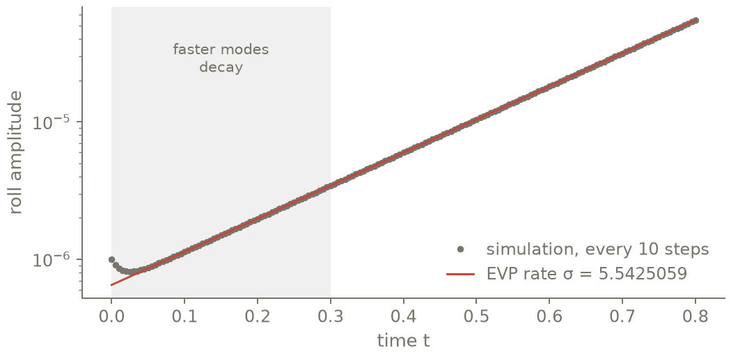
The initial-value problem against the eigenvalue problem. After t = 0.3 the amplitude grows at σ = 5.5425080, the EVP’s 5.5425059: a relative difference of 4×10⁻⁷, within the 10⁻⁵ the script checks.

A run over several jobs

A cluster job has a time limit, so a long run is a chain of jobs, and each job runs the same script. sim.resume_or_start(directory, T=...) continues from the latest checkpoint of directory when there is one and starts from the initial state otherwise; checkpoints writes exact restart files; output writes the fields and numbers you ask for. Without mode=, the output file is created on a fresh start (an existing one is refused rather than replaced: give mode="w" to replace it) and continued after a restart (rows written after the checkpoint are dropped and written again by the restarted run).

import tempfile
from pathlib import Path

work = Path(tempfile.mkdtemp(prefix="rb_chain_"))   # a real run: a directory of your project space


def job(until):
    """The script of every job of a chain: the same lines for the first job and the next ones."""
    sim = m.simulate(N=(16, 24), scheme="RK443", dt=5e-4)
    # the latest checkpoint of chk/ if there is one, else this initial state at t = 0
    sim.resume_or_start(work / "chk",
                        T=lambda x, z: -z + 1e-6 * np.cos(np.pi * x) * np.cos(np.pi * z))
    sim.checkpoints(work / "chk", every=200, keep=2)          # exact restart files
    sim.output(work / "rb.h5", every=100,                     # no mode=: follows the branch
               tasks={"T": "T", "KE": lambda s: s.evaluate("integ(u@u)/2")})
    sim.run(until=until)
    return sim


job(0.3)                                     # first job: from t = 0, stopped at t = 0.3
chain = job(0.8)                             # next job: from the checkpoint of t = 0.3
print("\n".join(s for s in chain.explain().splitlines() if "resume_or_start" in s))
d = cn.io.read(work / "rb.h5")               # also readable with h5py alone
print(f"{len(d.sim_time)} rows, t = {d.sim_time[0]:.2f} ... {d.sim_time[-1]:.2f}, "
      f"kinetic energy at the end {d.tasks['KE'][-1]:.3e}")

explain() says which branch was taken and which mode each file got. The chain gives the state of the uninterrupted run above bit for bit (checked below), because a checkpoint holds the state, the scheme’s history and the clock. More in Input and output (what an analysis file holds, mode=, the formats).

Check. EVP: \(\sigma = 5.5425059231\) (the streamfunction formulation gives \(5.542505923\)); IVP from a \(10^{-6}\) perturbation: \(\sigma = 5.5425080\) over \(t \in [0.3, 0.8]\), i.e. \(4\times10^{-7}\) relative.

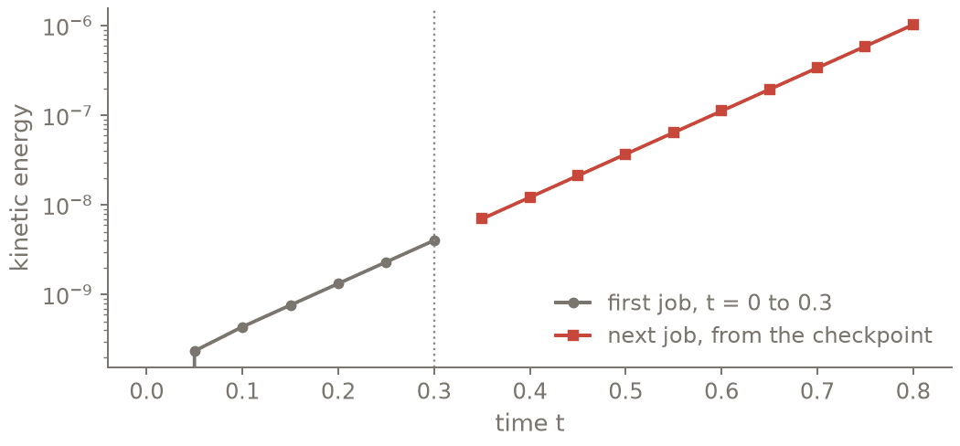
The kinetic energy written to rb.h5 by the two jobs of the chain: the second starts from the checkpoint of the first and continues the same file. One run, bit for bit.

SIGMA = 5.5425059                            # EVP of the same equations (tests/ivp/test_psi_theta.py)
assert abs(sigma_evp - SIGMA) < 1e-6, sigma_evp
assert abs(sigma_ivp - sigma_evp) < 1e-5, (sigma_ivp, sigma_evp)
assert np.array_equal(chain.solver.X, sim.solver.X) and len(d.sim_time) == 17   # two jobs = one run (t = 0 row included)
print("OK: the IVP grows at the EVP rate; the EVP matches the psi-theta formulation; the two-job "
      "chain is the uninterrupted run bit for bit")

Output (as executed)

# t02a_rayleigh_benard_cpu: PASS (exit 0) in 32.2 s | 2026-10-20 | script sha256 90eb240188d497ff
Model 'Rayleigh-Benard 2D': Box(x=periodic((0, 2)), z=walls(-0.5, 0.5)) (Cartesian box)
Unknowns: u (velocity), p (pressure), T (scalar); parameters: Ra = 2500, Pr = 1
Equations as written:
  momentum: dt(u) + grad(p) - Pr*lap(u) = Pr*Ra*T*ez - u·grad(u)
  continuity: div(u) = 0
  heat: dt(T) - lap(T) = -u·grad(T)
Problem: IVP (a time derivative dt() appears)
Time stepping: 7 linear term(s) implicit; nonlinear terms explicit (momentum, heat)
Boundary conditions: bottom: u = 0, T = 0.5; top: u = 0, T = -0.5 (tau method, placed automatically)
Gauge: the mean of p is fixed (integ(p) = 0)
Dealiasing: x: 3/2, z: 3/2 (declared default for products of degree 2)
Resolution: not chosen yet (simulate/eigenvalues/discretize(N=...))
(every decision, tau by tau and term by term: m.explain(full=True))
Linearization of 'Rayleigh-Benard 2D' about a base state, eigenvalue s (normal modes exp(s t)):
  u = 0 about the zero field
  T = T0(z), a non-constant coefficient
  base state: steady residual 0.0e+00 (largest relative residual of the equations and boundary conditions at the base, fitted by least squares: p, the automatic boundary terms; worst: -): a steady solution to BASE_RESIDUAL_TOL = 1e-06
  Fourier sizes chosen to hold k: N_x = 4 (the matrices of one wavenumber do not depend on the others)
EVP: growth rate of the k = pi roll at Ra = 2500: sigma = 5.5425059231
Simulation of 'Rayleigh-Benard 2D' at N = x: 16, z: 24: RK443, dt = 0.0005, backend cpu
  operators assembled (kept for reuse by the next identical simulate(); cache of 2 per model)
Parameters in use (compiled into this simulation): Ra = 2500, Pr = 1
Problem: IVP (a time derivative dt() appears)
Time stepping: 7 linear term(s) implicit; nonlinear terms explicit (momentum, heat)
Boundary conditions: bottom: u = 0, T = 0.5; top: u = 0, T = -0.5 (tau method, placed automatically)
Gauge: the mean of p is fixed (integ(p) = 0)
Dealiasing: x: 3/2, z: 3/2 (declared default for products of degree 2)
Initial state: T given; u, p start at zero
IVPSolver(scheme=RK443, dt=0.0005, constant step, backend=cpu)
  scheme: RK443: IMEX Runge–Kutta (4 stages), implicit L-stable SDIRK3 on L, explicit 4-stage Runge–Kutta on F; global order 3 (Ascher, Ruuth & Spiteri 1997, (4,4,3))
  finite-state check: every 100 steps (default), at the end of each run call and before each checkpoint/output write (NaN/inf -> NumericalError naming step, time and unknown; check_finite=False turns it off)
  resolution check: with the finite-state check, the relative spectral tail of each unknown and direction above 0.001 warns once (none so far)
(every decision, tau by tau and term by term, and the solver layout: sim.explain(full=True))
CFL time step at safety 0.5: 2.18e+01  (a stability indicator, not an error)
IVP: measured growth rate sigma = 5.5425080071 over t in [0.30, 0.80]
Methods paragraph generated from the plan (edit before publishing):

The IVP 'Rayleigh-Benard 2D' for (u, p, T) was solved with Conatus. The domain is discretized as follows: x ∈ [0, 2) is periodic and expanded in a real (cosine/sine) Fourier series of 16 modes; z ∈ [-0.5, 0.5] is expanded in 24 Chebyshev polynomials of the first kind. Derivatives, basis conversions and multiplications by non-constant coefficients use the sparse, banded ultraspherical operators of Olver & Townsend, and boundary conditions are imposed with the generalized tau method (4 tau variable(s), each entering through a lift polynomial), following Burns et al. The Fourier directions decouple, giving 8 independent systems, one per wavenumber. Nonlinear terms are evaluated pseudospectrally with dealiasing factors 3/2 in x, 3/2 in z. The structural rank of every system was checked before factorization. Time integration uses the third-order, four-stage IMEX Runge–Kutta scheme (4,4,3) of Ascher, Ruuth & Spiteri, whose implicit diagonal is constant so that a single factorization serves all stages, with a constant step Δt = 0.0005. The implicit systems are solved by banded LU factorization with a low-rank (Woodbury) correction for the tau rows, batched over wavenumbers on CPU, in float64 arithmetic. The equations were declared in the native layer of Conatus as written on paper; the implicit-explicit split, the 4 tau term(s) (each in the equation where its unknown has its highest wall-normal order) and the pressure gauge and its integral constraint were placed by fixed, declared rules (listed by explain()). The dealiasing factor 3/2 is the declared default of the native layer ((p+1)/2 for the highest polynomial degree p = 2 of the equations in the unknowns and given fields, at least 3/2).

Citations: olver2013, burns2020, ascher1997
Facts used: kind=IVP, groups=8, N_x=16, N_z=24, zbasis=Chebyshev, taus=4, dealias={'x': 1.5, 'z': 1.5}, scheme=RK443, dt=0.0005, backend=cpu, native=True, dealias_default=True
resume_or_start('<path>/rb_chain_60ae2ffv/chk'): continued from checkpoint_000000600.h5 (iteration 600, t = 0.3); outputs without mode= continue their file (mode='resume')
AnalysisFile <path>/rb_chain_60ae2ffv/rb.h5 (HDF5, conatus.analysis/1): every 100 steps (= 0.05 time units), 17 write(s) so far [mode 'resume' chosen by resume_or_start (restart)]
17 rows, t = 0.00 ... 0.80, kinetic energy at the end 1.028e-06
OK: the IVP grows at the EVP rate; the EVP matches the psi-theta formulation; the two-job chain is the uninterrupted run bit for bit

The same run on a GPU

The model does not change. Only the backend is chosen, explicitly: backend="cuda" in m.simulate(...) moves the state, the batched banded solves and the transforms to the device; f_backend="fused" evaluates the nonlinear terms with fused kernels (the NumPy "evaluator" remains the oracle). sim.solver.run_graph(n) captures one step as a CUDA graph and replays it, which removes the launch latency.

runs, early = {}, {}
for label, kw in [("cpu", dict(backend="cpu")),
                  ("gpu", dict(backend="cuda", f_backend="fused"))]:   # both choices explicit
    s = m.simulate(N=(128, 64), scheme="RK443", dt=2e-4, **kw)
    s.initial(T=T_init)
    s.run(steps=20)                                  # compare here: rounding not yet amplified
    early[label] = s.grid("T").copy()
    t0 = time.perf_counter()
    s.run(steps=180)                                 # timing (the flow becomes strongly nonlinear)
    runs[label] = (s, (time.perf_counter() - t0) / 180)
    print(f"{label}: {1e3 * runs[label][1]:.2f} ms per step")
print(runs["gpu"][0].explain())

g = m.simulate(N=(128, 64), scheme="RK443", dt=2e-4, backend="cuda", f_backend="fused")
g.initial(T=T_init)
g.solver.run_graph(20)                               # expert: capture one step, replay it
graph_early = g.grid("T").copy()
t0 = time.perf_counter()
g.solver.run_graph(180)
print(f"gpu + CUDA graph: {1e3 * (time.perf_counter() - t0) / 180:.2f} ms per step")

Tc, Tg = early["cpu"], early["gpu"]
diff_gpu = np.abs(Tc - Tg).max() / np.abs(Tc).max()
diff_graph = np.abs(graph_early - Tg).max() / np.abs(Tg).max()
late = np.abs(runs["cpu"][0].grid("T") - runs["gpu"][0].grid("T")).max()
print(f"after 20 steps: relative max |T_cpu - T_gpu| = {diff_gpu:.1e}; graph vs plain = {diff_graph:.1e}")
print(f"after 200 steps: max |T_cpu - T_gpu| = {late:.1e} (rounding amplified by the instability)")
assert diff_gpu <= 1e-11 and diff_graph <= 1e-13
print("OK: CPU and GPU agree to rounding; the graph replay is the same computation")

CPU and GPU are not bitwise equal (different summation orders), so the check is agreement to rounding, the cross-backend model of the test suite, and it is made early (20 steps). At \(Ra = 10^5\) the conduction state is violently unstable: the linearized problem has growth rates up to \(\sigma \approx 225\) (wavenumber \(2\pi\)), and the flow saturates nonlinearly within the 200 steps. Any rounding difference is amplified with it: after 200 steps two CPU evaluations of the same nonlinear terms (NumPy evaluator vs fused kernels) differ by \(4\times10^{-6}\), as do CPU and GPU. Comparing trajectories of an unstable flow needs a time horizon, stated with the tolerance.

Check. After 20 steps CPU and GPU (fused kernels) agree to \(1.0\times10^{-14}\) relative; the CUDA-graph replay equals plain GPU steps exactly.

Output (as executed, one L40S)

# t02b_rayleigh_benard_gpu: PASS (exit 0) in 14.5 s | 2026-10-02
cpu: 27.98 ms per step
gpu: 0.61 ms per step
Simulation of 'Rayleigh-Benard 2D' (native model) at N = x: 128, z: 64
Problem kind: IVP (a time derivative dt() appears)
Term placement (IMEX split, automatic; override with implicit(...) / explicit(...)):
  [0] momentum
      implicit  grad(p)   (linear, constant coefficients)
      implicit  -Pr*lap(u)   (linear, constant coefficients)
      implicit  dt(u)   (linear, constant coefficients)
      explicit  -dot(u, grad(u))   (nonlinear, degree(s) [2] in the unknowns)
      implicit  -Ra*Pr*T*ez   (linear, constant coefficients; moved from the right side)
  [1] continuity
      implicit  div(u)   (linear, constant coefficients)
  [2] heat
      implicit  dt(T)   (linear, constant coefficients)
      implicit  -lap(T)   (linear, constant coefficients)
      explicit  dot(-u, grad(T))   (nonlinear, degree(s) [2] in the unknowns)
Boundary conditions -> tau terms (automatic, deterministic):
  u = 0 at bottom: tau_u1 lifted into mode 63 (N_z-1) of [0] momentum -- u has its highest z-order (2) there; Chebyshev lift into the last modes
  u = 0 at top: tau_u2 lifted into mode 62 (N_z-2) of [0] momentum -- u has its highest z-order (2) there; Chebyshev lift into the last modes
  T = 0.5 at bottom: tau_T1 lifted into mode 63 (N_z-1) of [2] heat -- T has its highest z-order (2) there; Chebyshev lift into the last modes
  T = -0.5 at top: tau_T2 lifted into mode 62 (N_z-2) of [2] heat -- T has its highest z-order (2) there; Chebyshev lift into the last modes
Incompressibility recognized: p enters only through grad(p) and has no condition; [1] continuity is its constraint (div(u), no time derivative):
  gauge tau tau_p (a constant) added to [1]; integral constraint integ(p) = 0 fixes the mean p
  divergence tau dot(ez, lift(tau_u2, z, -1)) (the velocity tau of the lowest lifted mode)
Dealiasing: x: 3/2, z: 3/2 (declared default 3/2 of the native layer; override with dealias=)
Bases: RealFourier(x, size=128, bounds=(0.0, 2.0), dealias=3/2); Chebyshev(z, size=64, bounds=(-0.5, 0.5), dealias=3/2)
Initial state: T given; u, p start at zero
IVPSolver(scheme=RK443, dt=0.0002, constant step, backend=cuda)
  scheme: RK443: IMEX Runge–Kutta (4 stages), implicit L-stable SDIRK3 on L, explicit 4-stage Runge–Kutta on F; global order 3 (Ascher, Ruuth & Spiteri 1997, (4,4,3))
GlobalSystem: 64 group(s), 33275 unknowns (full space), dtype float64, ordering=interleaved, complexify=False
  2 solver bucket(s) (groups sharing one sparsity pattern, batched GPU bordered banded solves, one warp per mode)
  [x: k=0] n=263, border rows=7, band kl=12 ku=18
  [x: k=3.14159] n=524, border rows=12, band kl=24 ku=37
  0 complexified bucket(s)
  state resident on the device (CuPy), pivot=partial
  solves: gather/scatter fused in the solve kernel, independent buckets on concurrent streams, level-scheduled sparse LU factors (same factors and per-row arithmetic as the band kernel)
  F: pseudospectral CuPy (GPU) evaluator, products on each basis' declared dealiased grid; linear solves: C++ bordered banded, batched per bucket
FusedRHS (polynomial form): 8 factors -> 3 outputs, real, one batched transform each way, one fused kernel
  factor u[0]
  factor dx^1u[0]
  factor dz^1u[0]
  factor u[1]
  factor dx^1u[1]
  factor dz^1u[1]
  factor dx^1T
  factor dz^1T
  eq 0[0]: 2 monomials
  eq 0[1]: 2 monomials
  eq 2: 2 monomials
  real projection on RealFourier grids checked: imaginary part <= 1e-13 relative, error otherwise (GPU: accumulated on the device, checked after each step / replayed block)
  derivatives of products are refused (no Leibniz rewrite); parameters frozen, recompiled when they change
  F: 2D RealFourier x Chebyshev pipeline (8 factors -> 3 outputs, grid 192 x 96): factors from X (one block per Fourier pair), cuFFT (Chebyshev DCT by length-M real FFTs (Makhoul), then x), fused products, cuFFT back, C^(lam) conversion into the stacked rows; ~10 kernels per evaluation; same numbers as the fused evaluator to FFT rounding
  step loop: Python loop over steps; step() launches every kernel from the host, run_graph(n) captures one step as a CUDA graph and replays it once per step (same kernels, same arithmetic; constant dt, F independent of t)
  per stage: RK stage right-hand side MX0 + sum dt a F - dt h L X in one kernel for real float64 states (M X and L X applied inside it, roundings identical to the array operations; timestep/lincomb.py), then the batched solve
gpu + CUDA graph: 0.67 ms per step
after 20 steps: relative max |T_cpu - T_gpu| = 8.6e-15; graph vs plain = 0.0e+00
after 200 steps: max |T_cpu - T_gpu| = 9.1e-07 (rounding amplified by the instability)
OK: CPU and GPU agree to rounding; the graph replay is the same computation

Going further

• Half the unknowns with a reflection symmetry: 3. Symmetries and symmetry subspaces.

• Checkpoints and exact restart (multistep history included): Reproducibility and provenance.