14. Coming from Dedalus
Write a convection cell as a Conatus model, read the same cell from a Dedalus script, and check that the two agree.
Goal. The onset of two-dimensional Boussinesq convection between a hot and a cold wall:
write it as a native Conatus model: equations as on paper, conditions by wall name, no tau terms;
give a Dedalus 3 script of the same cell to
cn.from_dedalusand read its line-by-line report;run the translation and compare it with the native model as the wall-normal resolution grows;
optionally, run the script with Dedalus itself and compare it with the translation.
Expected. The report has no unsupported line. The native model and the translation are two
tau formulations of the same equations, so they differ by a truncation error that decays
spectrally with \(N_z\), down to rounding at \(N_z = 32\). With Dedalus installed, the check script
finds the translation equal to Dedalus to rounding (\(< 10^{-10}\) relative after 40 steps of
SBDF2).
Time: about 5 s of CPU; the Dedalus check takes under a minute, most of it importing Dedalus.
Scripts: t14_from_dedalus.py (no Dedalus needed),
rb_cell_dedalus.py (the Dedalus script, written for this tutorial),
t14b_dedalus_check.py (the comparison with Dedalus).
Tests behind it: tests/translate/, tests/parse/.
Guide: Coming from Dedalus, Equations.
The cell as a native model
# Onset of convection in diffusive units: th is the temperature minus the conduction profile 1 - z,
# so it vanishes on both walls; u.ez carries the conduction profile into the heat equation.
RA, PR, PERIOD, NX, DT = 3000.0, 7.0, 2.0, 24, 5e-4


def start(x, z):
    """One roll of the temperature deviation."""
    return 1e-3 * np.cos(2 * np.pi * x / PERIOD) * np.sin(np.pi * z)


def native(nz):
    """The cell as a Conatus model: unknowns by role, equations as written on paper, conditions by
    wall name. No tau field and no lift: the native layer places one tau per condition."""
    m = cn.Model(cn.Box(x=cn.periodic(PERIOD), z=cn.walls(0, 1)), name="convection onset",
                 Ra=RA, Pr=PR)
    m.velocity("u"), m.pressure("p"), m.scalar("th")
    m.equations("""
        momentum:  dt(u) - Pr*lap(u) + grad(p) - Ra*Pr*th*ez = -u·grad(u)
        mass:      div(u) = 0
        heat:      dt(th) - lap(th) - u·ez = -u·grad(th)
    """)
    m.at("bottom", u=0, th=0)
    m.at("top", u=0, th=0)
    sim = m.simulate(N=(NX, nz), scheme="SBDF2", dt=DT)
    sim.initial(th=start)
    return sim.run(steps=40)


cell = native(16)
print(f"native model: t = {cell.t:.3f}, max|u| = {np.abs(cell.grid('u')).max():.3e}")
You name the unknowns by their role and write the equations as you would on paper; lap, div
and grad are the operators of the box’s coordinates. The unknown th is the temperature minus
the conduction profile \(1 - z\), so it vanishes on both walls, and u·ez is the advection of that
profile; lengths are in units of the depth and times of the thermal diffusion time. The walls are bottom and top. There is
no tau field and no lift: the native layer adds one tau term per wall condition by a fixed rule,
which explain() prints.
The same cell in Dedalus
rb_cell_dedalus.py is the script a Dedalus user would write for this
cell. It reduces the equations to first order, so it declares the tau fields and the lifts
itself:
plane = d3.CartesianCoordinates('x', 'z')
mesh = d3.Distributor(plane, dtype=np.float64)
horiz = d3.RealFourier(plane['x'], size=N_x, bounds=(0, period), dealias=1.5)
vert = d3.ChebyshevT(plane['z'], size=N_z, bounds=(0, 1), dealias=1.5)
u = mesh.VectorField(plane, name='u', bases=(horiz, vert))
p = mesh.Field(name='p', bases=(horiz, vert))
th = mesh.Field(name='th', bases=(horiz, vert))
u_bot = mesh.VectorField(plane, name='u_bot', bases=horiz)    # tau terms, one per wall condition
u_top = mesh.VectorField(plane, name='u_top', bases=horiz)
th_bot = mesh.Field(name='th_bot', bases=horiz)
th_top = mesh.Field(name='th_top', bases=horiz)
gauge = mesh.Field(name='gauge')                               # constant tau of the pressure

# Tau terms live in the first-derivative basis of z; the bottom ones enter through the gradients
e_x, e_z = plane.unit_vector_fields(mesh)
dz_basis = vert.derivative_basis(1)
tau_z = lambda f: d3.Lift(f, dz_basis, -1)  # noqa: E731 (a Dedalus idiom)
Gu = d3.grad(u) + e_z*tau_z(u_bot)
Gth = d3.grad(th) + e_z*tau_z(th_bot)

onset = d3.IVP([u, p, th, u_bot, u_top, th_bot, th_top, gauge], namespace=locals())
onset.add_equation("dt(u) - Pr*div(Gu) + grad(p) - Ra*Pr*th*e_z + tau_z(u_top) = -u@grad(u)")
onset.add_equation("trace(Gu) + gauge = 0")
onset.add_equation("dt(th) - div(Gth) - u@e_z + tau_z(th_top) = -u@grad(th)")
onset.add_equation("u(z=0) = 0")
onset.add_equation("th(z=0) = 0")
onset.add_equation("u(z=1) = 0")
onset.add_equation("th(z=1) = 0")
onset.add_equation("integ(p) = 0")

# Fixed-step SBDF2 run from one roll of the deviation
run = onset.build_solver(d3.SBDF2)
run.stop_iteration = steps
x, z = mesh.local_grids(horiz, vert)
th['g'] = 1e-3*np.cos(2*np.pi*x/period)*np.sin(np.pi*z)
while run.proceed:
    run.step(tstep)
It uses a fixed time step and a deterministic start. Conatus never adapts dt by itself, and
fill_random cannot be repeated outside Dedalus. Given a script with a CFL or a fill_random
line, the translator marks that line unsupported and says what to write instead.
Translate and read the report
SCRIPT = os.path.join(os.path.dirname(os.path.abspath(__file__)), "rb_cell_dedalus.py")
tr = cn.from_dedalus(SCRIPT)          # read with `ast`, never executed; Dedalus is not imported
print(tr.explain())
counts = tr.counts()
The script is parsed with ast and read statement by statement by a restricted interpreter.
Nothing in it is executed, and Dedalus is not imported. In the output below, look for:
e_z*tau_z(u_bot): a product of two vectors, which Dedalus reads as a tensor product. The report saysouter.trace(Gu): it becomesdiv(u)plus the tau term, anddiv(outer(ez, ...))becomesdz(...). Both are exact identities, and both are listed.dealias=1.5, written in the script. When a script leavesdealiasout, the translator writes the Dedalus default of 1 explicitly and reports it.The
whileloop: it becomessolver.run(n)with the script’s fixeddt.
Run the translation
solver = tr.ivp_solver(startup="lower_order")      # the script's SBDF2, dt and initial th
solver.run(tr.steps())                              # 40 steps, no Python time loop
print(f"translation: t = {solver.t:.3f} after {tr.steps()} steps, "
      f"max|u| = {np.abs(solver.grid('u')).max():.3e}")
tr.ivp_solver takes the script’s scheme and dt, and replays its th['g'] = ... line on the
Conatus grid. SBDF2 is a two-step scheme: startup="lower_order" is the start-up Dedalus uses
(one first-order step), written here explicitly.
Native model and translation, side by side
def translated(nz):
    """The same script at another wall-normal resolution (a declared, reported override)."""
    t = cn.from_dedalus(SCRIPT, overrides={"N_z": nz})
    s = t.ivp_solver(startup="lower_order")
    s.run(t.steps())
    return s


def rel(a, b, name):
    return np.abs(a.grid(name) - b.grid(name)).max() / np.abs(b.grid(name)).max()


gap = {}
for nz in (12, 16, 32):
    a, d = (cell, solver) if nz == 16 else (native(nz), translated(nz))
    gap[nz] = (rel(a, d, "th"), rel(a, d, "u"))
    print(f"nz = {nz:2d}: native vs translated, relative difference th {gap[nz][0]:.1e}, "
          f"u {gap[nz][1]:.1e}")
The translation keeps the script’s tau terms; the native model places its own. These are two
discretisations of the same equations, so they agree up to the truncation error, not to
rounding. The difference falls spectrally as \(N_z\) grows and reaches rounding at \(N_z = 32\):
both converge to the same solution, and the difference measures how far the coarser grids are
from it. overrides={"N_z": nz} changes one top-level assignment of the script, and the report
lists the change.
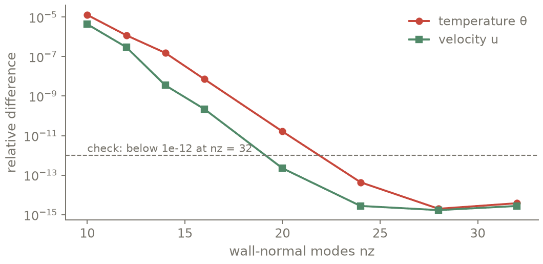
Native model against the translated Dedalus script after 40 SBDF2 steps: two tau formulations of the same equations, whose difference falls spectrally with nz down to rounding.
Compare with Dedalus
t14b_dedalus_check.py runs the same file with Dedalus, if
Dedalus is installed (micromamba install -c conda-forge dedalus), and compares the result with
the translation:
os.environ.setdefault("OMP_NUM_THREADS", "1")      # Dedalus asks for it before its import
try:
    import dedalus  # noqa: F401  (comparison oracle only; the conatus package never imports it)
    have_dedalus = True
except ImportError:
    have_dedalus = False
    print("Dedalus is not installed here: the comparison with Dedalus is skipped (declared)")

if have_dedalus:
    logging.disable(logging.INFO)                   # Dedalus's per-step log lines
    ns = runpy.run_path(SCRIPT, run_name="__main__")   # the script, run by Dedalus as written
    out = {}
    for name in ("th", "u"):
        ns[name].change_scales(1)                   # back to the grid without 3/2 padding
        out[name] = np.array(ns[name]["g"])
    rel_th = np.abs(out["th"] - th_cn).max() / np.abs(out["th"]).max()
    rel_u = np.abs(out["u"] - u_cn).max() / np.abs(out["u"]).max()
    print(f"Dedalus: t = {ns['run'].sim_time:.3f}; relative difference th {rel_th:.1e}, "
          f"u {rel_u:.1e}")
Both codes now use the same method: the same bases, tau terms, lifts, scheme, start-up and dealiasing. So the difference is rounding.
Output (as executed)
# t14_from_dedalus: PASS (exit 0) in 10.8 s | 2026-10-20 | script sha256 fe7119efa6854020
native model: t = 0.020, max|u| = 4.225e-02
Dedalus -> Conatus: rb_cell_dedalus.py
  39 translated, 0 approximated, 0 unsupported, 0 skipped (output only)
  problem: IVP with 8 equations, variables u, p, th, u_bot, u_top, th_bot, th_top, gauge
  time stepping: SBDF2, dt = 0.0005, stop_sim_time = None; ivp_solver() imposes time-dependent boundary data as Dedalus does (bc_time='step'; bc_time='auto' for the Conatus default, which keeps the order of the scheme)
  data: th (translated)
Line-by-line report:
  20  translated   import numpy as np
  21  translated   import dedalus.public as d3
  24  translated   Ra = 3000.0
  25  translated   Pr = 7.0
  26  translated   period = 2.0
  27  translated   N_x, N_z = 24, 16
  28  translated   tstep = 5e-4
  29  translated   steps = 40
  32  translated   plane = d3.CartesianCoordinates('x', 'z')
  33  translated   mesh = d3.Distributor(plane, dtype=np.float64)
  34  translated   horiz = d3.RealFourier(plane['x'], size=N_x, bounds=(0, period), de...
  35  translated   vert = d3.ChebyshevT(plane['z'], size=N_z, bounds=(0, 1), dealias=1.5)
  36  translated   u = mesh.VectorField(plane, name='u', bases=(horiz, vert))
  37  translated   p = mesh.Field(name='p', bases=(horiz, vert))
  38  translated   th = mesh.Field(name='th', bases=(horiz, vert))
  39  translated   u_bot = mesh.VectorField(plane, name='u_bot', bases=horiz)
  40  translated   u_top = mesh.VectorField(plane, name='u_top', bases=horiz)
  41  translated   th_bot = mesh.Field(name='th_bot', bases=horiz)
  42  translated   th_top = mesh.Field(name='th_top', bases=horiz)
  43  translated   gauge = mesh.Field(name='gauge')
  46  translated   e_x, e_z = plane.unit_vector_fields(mesh)
  47  translated   dz_basis = vert.derivative_basis(1)
  48  translated   tau_z = lambda f: d3.Lift(f, dz_basis, -1)
  49  translated   Gu = d3.grad(u) + e_z*tau_z(u_bot)
                  -> 'ez*lift(u_bot, z, -1, lam=1)' of two tensors -> outer (Dedalus convention)
  50  translated   Gth = d3.grad(th) + e_z*tau_z(th_bot)
  52  translated   onset = d3.IVP([u, p, th, u_bot, u_top, th_bot, th_top, gauge], nam...
  53  translated   onset.add_equation("dt(u) - Pr*div(Gu) + grad(p) - Ra*Pr*th*e_z + t...
                  -> div(outer(ez, lift(u_bot, z, -1, lam=1))) -> dz(lift(u_bot, z, -1, lam=1)) (exact identity, constant unit vector)
  54  translated   onset.add_equation("trace(Gu) + gauge = 0")
                  -> trace(outer(ez, lift(u_bot, z, -1, lam=1))) -> dot(...) (exact identity); trace(grad(u)) -> div(u) (exact identity); namespace functions used: trace
  55  translated   onset.add_equation("dt(th) - div(Gth) - u@e_z + tau_z(th_top) = -u@...
  56  translated   onset.add_equation("u(z=0) = 0")
  57  translated   onset.add_equation("th(z=0) = 0")
  58  translated   onset.add_equation("u(z=1) = 0")
  59  translated   onset.add_equation("th(z=1) = 0")
  60  translated   onset.add_equation("integ(p) = 0")
  63  translated   run = onset.build_solver(d3.SBDF2)
                  -> solver: IVPSolver(plan, 'SBDF2', dt) (dt from the time loop)
  64  translated   run.stop_iteration = steps
                  -> number of steps: solver.run(n)
  65  translated   x, z = mesh.local_grids(horiz, vert)
                  -> grid coordinates: used for initial / given data only
  66  translated   th['g'] = 1e-3*np.cos(2*np.pi*x/period)*np.sin(np.pi*z)
                  -> grid data of th: initial condition / given field (tr.data)
  67  translated   while run.proceed:
                  -> time loop -> solver.run(n) with a fixed dt = 0.0005 (no Python loop); the loop body (logging, analysis) is not translated
translation: t = 0.020 after 40 steps, max|u| = 4.225e-02
nz = 12: native vs translated, relative difference th 1.2e-06, u 3.0e-07
nz = 16: native vs translated, relative difference th 7.2e-09, u 2.2e-10
nz = 32: native vs translated, relative difference th 3.8e-15, u 2.8e-15
PASS
The Dedalus check:
# t14b_dedalus_check: PASS (exit 0) in 21.8 s | 2026-10-20 | script sha256 763cece2d005a63e
Conatus: t = 0.020 after 40 steps
2026-10-20 13:30:36,614 dedalus 0/1 WARNING :: Threading has not been disabled. This may massively degrade Dedalus performance.
2026-10-20 13:30:36,614 dedalus 0/1 WARNING :: We strongly suggest setting the "OMP_NUM_THREADS" environment variable to "1".
Dedalus: t = 0.020; relative difference th 3.0e-14, u 3.8e-15
PASS
Going further
print(tr.to_script())writes a runnable Conatus program (it replays the translation and runs it), with the report as comments.For a problem built inside a function, use
cn.from_dedalus(script, entry=("f", {...})).Coming from Dedalus lists the translated subset and the comparisons on the official Dedalus examples. These include KdV–Burgers (1.3e-15), Poisson (7e-16), shear flow (1.3e-15), the Rayleigh–Bénard eigenvalue problem (4e-16) and the pipe-flow eigenvalues on the disk (5e-14).