Getting started in ten minutes

1. Install

$ python3.12 -m venv venv && . venv/bin/activate
$ pip install "conatus[tutorials]"
$ python -m conatus doctor

The last line says what this machine can run; Installation has the other ways to install.

2. The equation

A wave u(x,t) on a periodic line of length 2π steepens under its own advection and is held back by viscosity ν:

import numpy as np

import conatus as cn

m = cn.Model(cn.Box(x=cn.periodic(2 * np.pi)), name="Burgers", nu=0.1)
m.scalar("u")
m.equations("dt(u) - nu*lap(u) = -u*dx(u)")
print(m.explain())

The domain, the unknown, the parameter and the equation are all you write. m.explain() prints what Conatus decided from them: the linear term is treated implicitly, the product u*dx(u) explicitly, and the product is dealiased by the 3/2 rule.

Time stepping: 2 linear term(s) implicit; nonlinear terms explicit (eq0)
Dealiasing: x: 3/2 (declared default for products of degree 2)

3. Simulate and plot

sim = m.simulate(N=128, scheme="RK443", dt=1e-3)    # resolution, scheme, time step: your choices
sim.initial(u=lambda x: np.sin(x))
x = sim.coordinate("x")
profiles = {}
for t in (0.0, 0.5, 1.0, 1.5, 2.0):
    if t > sim.t:
        sim.run(until=t)
    profiles[t] = sim.grid("u").copy()

A simulation needs a resolution, a scheme and a time step: three arguments, never defaults. run(until=t) advances to t, which must be a whole number of steps: the step is never changed for you.

import os

import matplotlib.pyplot as plt

fig, ax = plt.subplots(figsize=(6.4, 3.2), dpi=150)
for t, ut in profiles.items():
    ax.plot(x, ut, label=f"t = {t:g}")
ax.set_xlabel("x")
ax.set_ylabel("u")
ax.legend(frameon=False)
out = os.environ.get("CN_TUTORIAL_OUT", ".")
os.makedirs(out, exist_ok=True)
fig.savefig(os.path.join(out, "burgers.png"), bbox_inches="tight")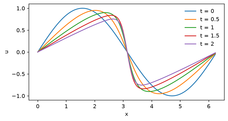

4. One physical number

The kinetic energy E = 1/2∫u² dx starts at π/2 and decreases as viscosity dissipates the steepening front.

u = sim.grid("u")
energy = np.pi * np.mean(u**2)                     # E = 1/2 int u^2 dx (grid mean, exact here)
print(f"kinetic energy at t = {sim.t:g}: E = {energy:.12f} (E(0) = pi/2 = {np.pi / 2:.12f})")

The Cole–Hopf transformation turns the Burgers equation into the heat equation, so the exact solution is known (Cole 1951; Hopf 1950). The script ends by comparing the energy with it:

kinetic energy at t = 2: E = 0.759907890109 (E(0) = pi/2 = 1.570796326795)
Cole-Hopf: E = 0.759907890081, relative error 3.7e-11
OK: the kinetic energy of the simulation equals the exact Cole-Hopf value

5. Four changes to try

Change one line of the script, run it again and read what happens.

1. Less viscosity. cn.Model(..., nu=0.05) makes the front twice as steep. The energy still matches the exact solution (change the 0.1 of cole_hopf_energy too), to 2×10⁻¹⁰.
2. Too few modes. m.simulate(N=32, ...) cannot resolve the front. Conatus does not raise the resolution for you: it warns, once, with an UnderResolvedWarning that names the unknown, the direction and the spectral tail, and the energy is then only right to about 4×10⁻⁶.
3. A larger time step. dt=0.05 takes 40 steps instead of 2000. The scheme is third order in time, so the energy error grows to about 4×10⁻⁶; sim.cfl(safety=0.5) tells you a stable step, it never imposes one.
4. Another equation. Drop the nonlinear term: m.equations("dt(u) - nu*lap(u) = 0") is the heat equation, and the energy decays exactly as E(t) = π/2e^−2νt.

6. Next

Getting started: convection between two plates takes one problem, convection between two plates, from its equations to its stability, its onset and a simulation; then each tutorial of Tutorials ends on a published value.

7. Output

Model 'Burgers': Box(x=periodic((0, 6.28319))) (Cartesian box)
Unknowns: u (scalar); parameters: nu = 0.1
Equations as written:
  eq0: dt(u) - nu*lap(u) = -u*dx(u)
Problem: IVP (a time derivative dt() appears)
Time stepping: 2 linear term(s) implicit; nonlinear terms explicit (eq0)
Dealiasing: x: 3/2 (declared default for products of degree 2)
Resolution: not chosen yet (simulate/eigenvalues/discretize(N=...))
(every decision, tau by tau and term by term: m.explain(full=True))
kinetic energy at t = 2: E = 0.759907890109 (E(0) = pi/2 = 1.570796326795)
Cole-Hopf: E = 0.759907890081, relative error 3.7e-11
OK: the kinetic energy of the simulation equals the exact Cole-Hopf value